Field Log · Entry

Embedding이란 무엇인가: 연구와 실전의 전체 지도 (1/14)

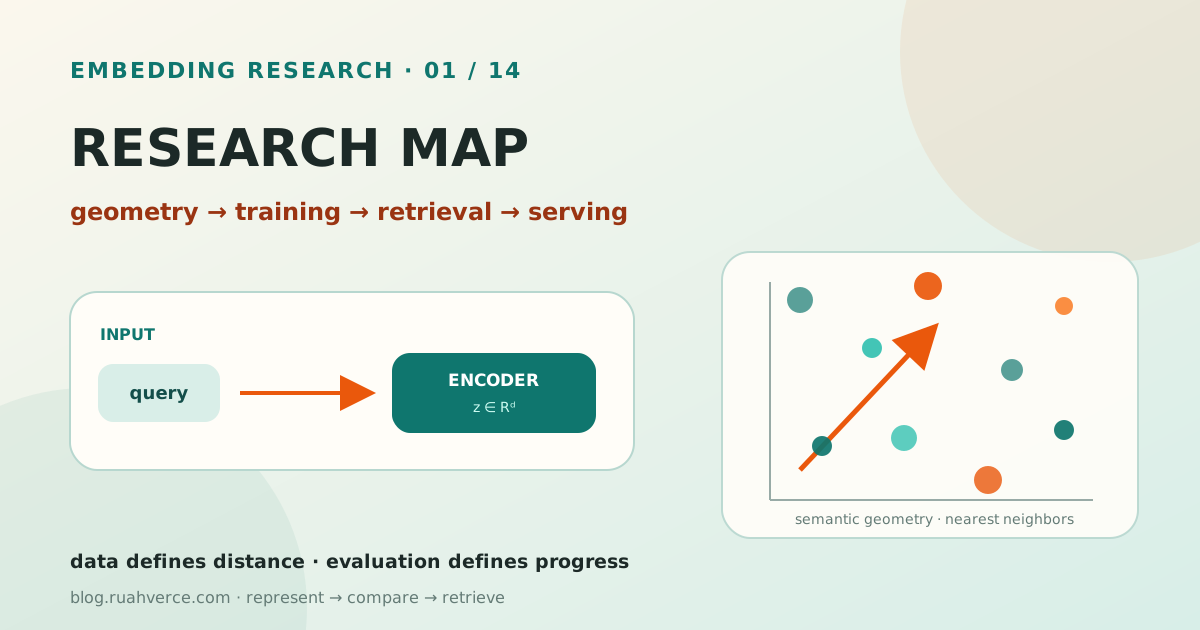
이번 글의 결론

• Embedding은 의미 그 자체가 아니라, 특정 학습 목표가 보존하라고 요구한 관계를 좌표로 압축한 표현입니다.
• “가까움”의 뜻은 model과 task가 정합니다. STS용 유사도, 검색 relevance, 분류 feature, recommendation affinity는 같은 공간을 요구하지 않습니다.
• Dense single-vector, learned sparse, multi-vector는 서로 배타적인 세대가 아니라 품질·저장·검색 비용을 바꾸는 표현 선택입니다.
• 연구는 data → encoder/pooling → objective → exact evaluation → ANN evaluation → downstream utility의 연결을 고정해야 재현됩니다.
• 공개 leaderboard는 shortlist 도구입니다. 최종 선택은 한국어·도메인·길이·비용을 반영한 in-domain 평가에서 합니다.

LLM과 RAG를 만들다 보면 embedding을 대개 한 줄로 처음 만납니다.

vectors = model.encode(texts)

하지만 이 한 줄 뒤에는 무엇을 비슷하다고 볼지, 어떤 차이를 버릴지, 어떤 negative에서 경계를 배울지, 수백만 vector 중 얼마나 정확히 찾을지에 관한 결정이 있습니다. 이 시리즈는 그 결정을 연구 가능한 단위로 해체합니다.

---

1. Embedding을 함수로 본다

Encoder (f_\theta)는 입력 (x)를 (d)차원 vector로 바꿉니다.

fθ: X → R^d
x  → z = [z1, z2, ..., zd]

검색에서는 query encoder와 document encoder가 같을 수도, 다를 수도 있습니다.

zq = fq(q)
zd = fd(d)
score(q, d) = sim(zq, zd)

중요한 것은 각 차원의 독립적인 뜻을 사람이 붙일 수 있다는 의미가 아닙니다. Model은 loss를 줄이는 데 유용한 관계적 geometry를 여러 차원에 분산해 저장합니다.

2. Word Vector와 Contextual Embedding은 다르다

고전적인 static word embedding에서는 같은 token이 대체로 같은 vector를 가집니다.

"은행에 돈을 맡겼다"의 은행 ─┐
                               ├─ same lookup vector
"강의 은행나무 옆"의 은행 ───┘

Contextual language model은 주변 token과 attention한 hidden state를 만듭니다.

token embedding + position
  → Transformer context
  → contextual token states h1...hT

Sentence/document embedding model은 이 token state들을 pooling하거나 특별 token을 사용해 고정 길이 vector로 압축합니다.

3. 표현 단위에 따른 분류

단위	출력	대표 용도	주요 손실
Token embedding	token마다 vector	tagging, late interaction	저장·비교 비용
Sentence embedding	문장당 vector	STS, clustering, dedup	긴 의미 압축
Passage embedding	chunk당 vector	dense retrieval, RAG	chunk boundary
Document embedding	문서당 vector	추천, coarse search	세부 근거 희석
Entity/item embedding	객체당 vector	recommendation, graph	cold-start·시간 변화
Multimodal embedding	text·image·video vector	cross-modal search	modality gap

한 model이 여러 단위를 지원한다고 해도 같은 품질을 보장하지 않습니다.

4. Dense·Sparse·Multi-vector

Dense Single-vector

한 입력을 수백~수천 차원의 실수 vector 하나로 표현합니다.

document → [0.12, -0.07, ..., 0.31]

장점은 고정 크기, 빠른 dot product, ANN index와의 결합입니다. 단점은 긴 입력의 여러 사실을 한 점에 압축한다는 것입니다.

Learned Sparse Vector

어휘 차원 대부분은 0이고 일부 token/term에 weight가 있습니다.

{"reranker": 2.1, "cross": 0.8, "encoder": 1.4}

Lexical match와 inverted index의 장점을 유지하면서 neural expansion을 학습할 수 있습니다.

Multi-vector

입력 하나에 token·patch·segment vector 여러 개를 저장하고 query와 late interaction합니다.

query:    q1 q2 ... qm
document: d1 d2 ... dn

score = Σ_i max_j sim(qi, dj)

ColBERT 설명처럼 세밀한 match를 보존하지만 vector 수와 검색 비용이 증가합니다.

Hybrid Output

BGE-M3처럼 한 model에서 dense, sparse, multi-vector representation을 함께 만들고 결합하는 계열도 있습니다. “embedding model = dense vector 하나”라는 정의는 이제 너무 좁습니다.

5. Symmetric Task와 Asymmetric Task

Symmetric

두 입력의 역할이 비슷합니다.

• paraphrase detection
• duplicate sentence
• 비슷한 상품끼리 찾기
• clustering

sim(f(x1), f(x2))

Asymmetric

Query는 짧은 정보 요구이고 document는 답을 담은 passage입니다.

"환불 기간은?" ↔ "구매 후 14일 이내 반품할 수 있습니다."

문자열도 길이도 역할도 다릅니다. E5 계열의 query: / passage: prefix, instruction-tuned embedding의 task prompt는 이 비대칭을 model에 알려 줍니다. Query와 document template을 뒤섞으면 같은 checkpoint도 크게 달라질 수 있습니다.

6. Bi-Encoder가 빠른 이유

Document vector를 offline에 미리 계산할 수 있습니다.

offline:
  documents → document encoder → vector index

online:
  query → query encoder → ANN top-N

Cross-Encoder는 query와 document를 함께 읽어 더 세밀하지만 corpus 전체에 적용하기 어렵습니다.

구조	document 사전 계산	query-document interaction	일반 역할
Bi-Encoder	가능	vector similarity만	first-stage retrieval
Cross-Encoder	불가	full attention	reranking
Late Interaction	token vector 사전 계산	token-level max similarity	retrieval/reranking 사이

그래서 embedding과 reranker는 경쟁자보다 cascade의 서로 다른 단계입니다.

7. Embedding이 보존해야 할 것은 Task가 정한다

같은 두 문장을 봅시다.

A: 이 약은 임산부에게 권장된다.
B: 이 약은 임산부에게 권장되지 않는다.

Topic clustering에서는 매우 가깝게 두어도 됩니다. Safety retrieval에서는 부정 하나가 결정적이므로 명확히 구분해야 합니다.

semantic relatedness ≠ task relevance ≠ entailment

“사람이 보기에 비슷한가?”만으로 embedding quality를 정의할 수 없는 이유입니다.

8. 어디에 쓰이는가

• semantic search와 RAG candidate retrieval
• recommendation·similar item
• clustering과 topic discovery
• classification의 frozen feature
• duplicate detection·entity resolution
• anomaly detection
• few-shot example retrieval
• memory retrieval for agents
• code search
• text↔image·page·video cross-modal search

각 용도는 query distribution, positive definition, metric이 다릅니다.

9. 연구 Pipeline의 단위

problem definition
  → corpus/query/label construction
  → encoder + pooling + input template
  → objective + batch/negative policy
  → exact vector evaluation
  → ANN/compression evaluation
  → downstream system evaluation
  → slice/error analysis

model A의 MTEB가 높다만으로 이 pipeline을 대체할 수 없습니다.

10. 세 종류의 품질 상한

Representation Ceiling

Exact nearest-neighbor에서도 relevant item이 가깝지 않다면 model 또는 data 문제입니다.

Index Ceiling

Exact top-k에는 있는데 ANN top-k에서 잃으면 index·quantization 문제입니다.

ANN recall@k = |ANN_top-k ∩ exact_top-k| / k

Corpus/Label Ceiling

Gold 문서가 corpus에 없거나 chunk가 답을 분리해 버리면 model이 되살릴 수 없습니다.

이 세 실패를 구분하지 않으면 HNSW parameter 문제를 fine-tuning으로 고치거나, 나쁜 label을 큰 model로 덮게 됩니다.

11. 첫 Baseline을 만드는 법

최소 실험은 다음 네 system이면 됩니다.

1. BM25
2. 공개 multilingual embedding + exact search
3. 같은 embedding + production ANN
4. hybrid BM25+dense

기록할 값:

baseline:
  corpus_snapshot: docs-2026-07-01
  queries: eval-v1
  model: pinned-model-revision
  prompt:
    query: "..."
    document: "..."
  pooling: official
  normalize: true
  dimension: 1024
  similarity: cosine
  search:
    exact: true
    ann_config: null
  metrics: [recall_at_10, recall_at_100, ndcg_at_10]

공식 model card의 prompt, pooling, normalization을 그대로 재현한 결과부터 시작합니다.

12. 14편 학습 순서

편	질문	결과물
1	Embedding 연구의 전체 범위는?	분류 지도와 baseline
2	Vector 거리와 pooling은 무엇을 바꾸나?	geometry 진단
3	Contrastive loss는 어떻게 공간을 만드나?	InfoNCE 실험
4	Positive·negative를 어떻게 설계하나?	data mining pipeline
5	Dense retrieval 학습은 어떻게 발전했나?	multi-stage recipe
6	Instruction·LLM backbone은 왜 쓰나?	input contract
7	Synthetic data·distillation로 어떻게 적응하나?	domain training plan
8	한국어·cross-lingual은 어떻게 평가하나?	multilingual matrix
9	긴 문서와 multi-vector를 어떻게 다루나?	contextual retrieval 설계
10	어떤 metric과 통계로 비교하나?	evaluation protocol
11	Benchmark를 어떻게 읽고 의심하나?	benchmark card
12	Dimension·quantization·ANN을 어떻게 묶나?	serving Pareto
13	2024–2026 연구는 어디로 가나?	research map
14	전 과정을 어떻게 재현하나?	end-to-end lab

13. 이 시리즈에서 지킬 원칙

• 공개 논문의 결과는 그 논문의 data·metric·시점에 한정해 서술합니다.
• API/leaderboard의 “현재 1위”를 영구 사실로 취급하지 않습니다.
• Exact와 ANN, model과 chunking, retrieval과 generation gain을 분리합니다.
• 한국어 성능을 multilingual 평균에서 추론하지 않고 직접 평가합니다.
• Vector도 원문만큼 민감할 수 있으므로 privacy·access control을 포함합니다.

스스로 확인하기

1. 같은 cosine similarity model이 clustering에는 적합하고 safety retrieval에는 부적합할 수 있는 이유는 무엇인가?
2. Bi-Encoder가 Cross-Encoder보다 corpus-scale 검색에 적합한 핵심 이유는 무엇인가?
3. Single-vector와 multi-vector의 가장 큰 비용 차이는 무엇인가?
4. Exact search와 ANN 결과를 분리해야 어떤 실패를 진단할 수 있는가?
5. Embedding model만 바꾸고 prompt·pooling·normalization을 기록하지 않으면 왜 재현이 어려운가?

다음 글에서는 cosine·dot product·L2, normalization, pooling, anisotropy와 hubness를 실제 검색 결과와 연결합니다.

참고자료

• Sentence-BERT: Sentence Embeddings using Siamese BERT-Networks
• Dense Passage Retrieval for Open-Domain Question Answering
• MTEB: Massive Text Embedding Benchmark
• BGE M3-Embedding
• ColBERTv2: Effective and Efficient Retrieval via Lightweight Late Interaction