Field Log · Entry

LLM 사전학습 목표와 Scaling Law: Token·Parameter·Compute 예산 (2/10)

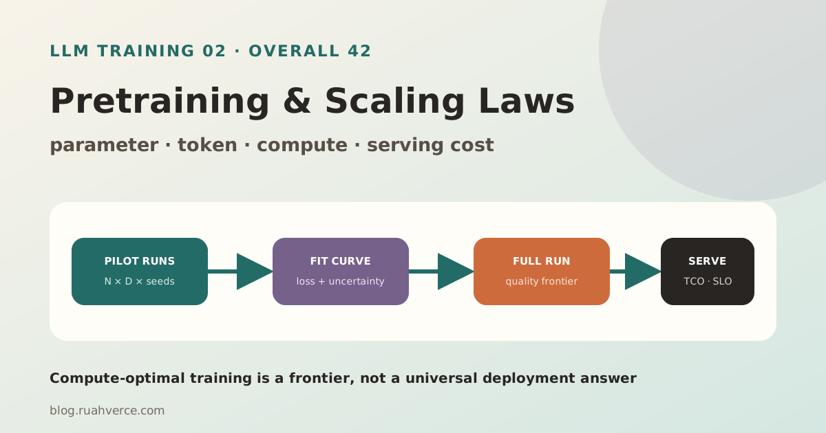
작은 pilot run의 parameter와 token별 loss를 scaling curve로 적합하고 training compute와 serving 비용을 함께 고려해 full run을 선택하는 구조

오늘의 결론

Decoder LLM의 기본 사전학습은 앞 token으로 다음 token의 확률을 맞히는 causal language modeling입니다.

Model parameter N, training token D, compute C는 독립적인 “크기 자랑” 지표가 아니라 고정 예산을 배분하는 변수입니다.

Kaplan과 Chinchilla의 scaling law는 경험적 관측입니다. 특정 token/parameter 비율을 모든 model과 data에 복사하는 법칙이 아닙니다.

Compute-optimal training과 production-optimal deployment는 목적 함수가 다릅니다. 많은 traffic에서는 작은 model을 더 오래 학습하는 편이 lifecycle cost에 유리할 수 있습니다.

Scaling fit은 작은 pilot grid, holdout 검증, 불확실성 구간, 안정성·downstream 평가와 함께 사용해야 합니다.

앞 글에서는 원시 문서가 versioned training shard가 되는 과정을 만들었습니다. 이제 그 token을 model에 넣습니다.

가장 단순한 질문은 이것입니다.

주어진 training compute를
  model parameter에 얼마나 쓰고,
  training token에 얼마나 쓰며,
  언제 학습을 멈출 것인가?

“가능한 가장 큰 model”도, “가능한 모든 data”도 자동으로 정답이 아닙니다.

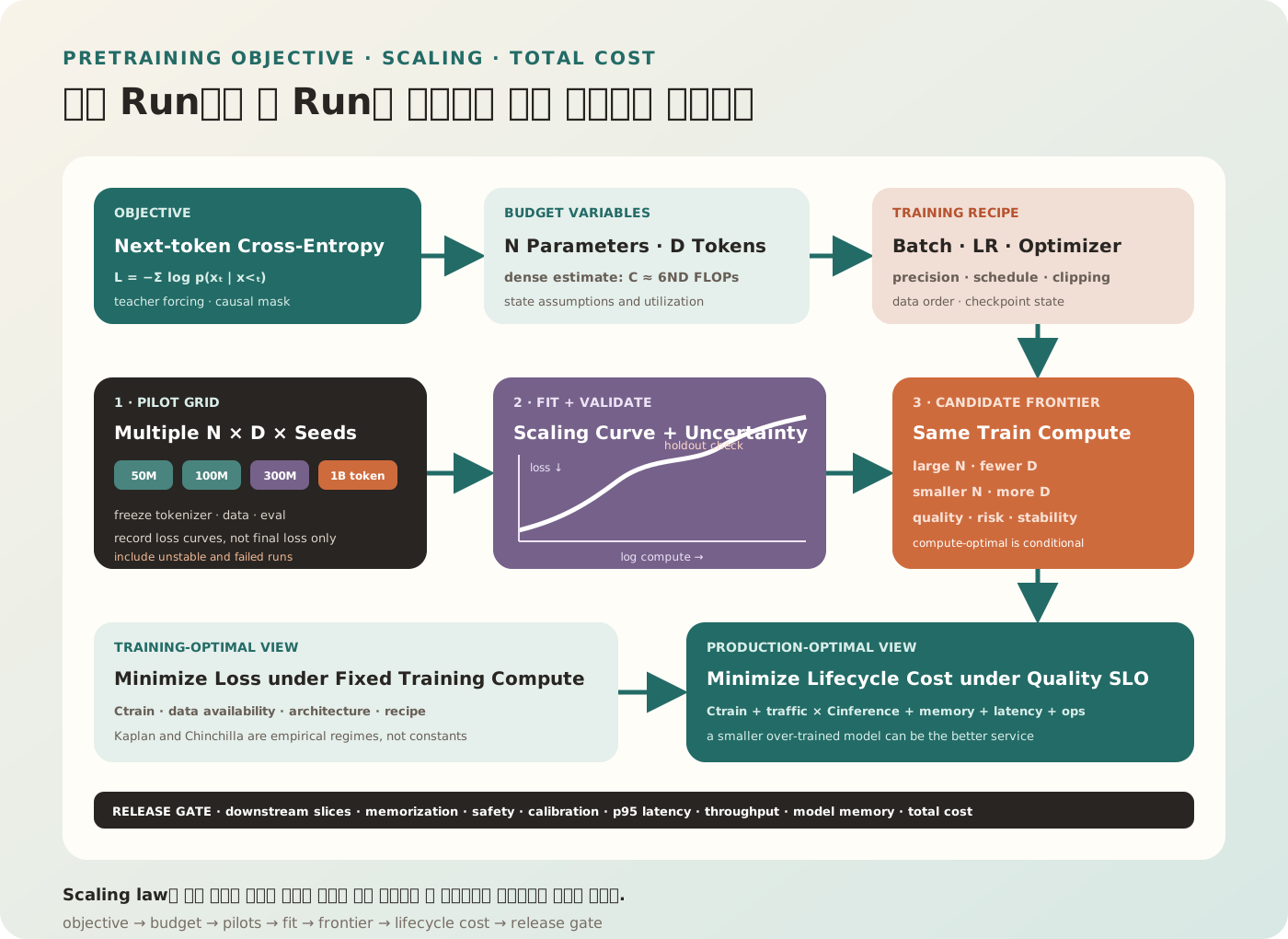
causal next-token objective에서 parameter token compute 예산과 pilot grid, scaling fit, training-optimal frontier, production lifecycle cost로 이어지는 의사결정 구조

그림 1. Scaling law는 작은 run의 loss curve로 후보를 줄이는 도구다. 실제 배포 model은 downstream quality, memory, traffic, latency를 포함한 별도의 목적 함수로 고른다.

사전학습이 실제로 푸는 문제

Token sequence를 다음처럼 둡니다.

x₁, x₂, x₃, ..., x_T

Autoregressive language model은 전체 sequence의 확률을 조건부 확률의 곱으로 분해합니다.

p(x₁, ..., x_T)
= Πₜ p(xₜ | x₁, ..., xₜ₋₁)

Training에서는 정답 prefix를 입력으로 주고 다음 token의 negative log-likelihood를 줄입니다.

L(θ)
= − Σₜ mₜ log pθ(xₜ | x₍<t₎)

θ: model parameter
mₜ: 해당 token의 loss를 계산할지 정하는 mask
x₍<t₎: 현재 token 앞의 prefix

Batch와 token 수로 평균하면 cross-entropy loss가 됩니다.

Teacher Forcing

Training step에서 model이 직전에 틀린 예측을 했더라도 다음 position 입력에는 dataset의 실제 token을 사용합니다.

input:   [오늘, 날씨, 는]
target:  [날씨, 는, 맑다]

이 방식을 teacher forcing이라고 부릅니다.

Causal Mask

Position t는 미래 token t+1 이후를 attention으로 보면 안 됩니다.

can attend?

        key position
query   1  2  3  4
  1     ✓  ×  ×  ×
  2     ✓  ✓  ×  ×
  3     ✓  ✓  ✓  ×
  4     ✓  ✓  ✓  ✓

미래 token이 보이면 training loss는 낮아지지만 generation과 같은 문제가 아닙니다.

Loss와 Perplexity

평균 cross-entropy가 L이면 perplexity는 보통 다음처럼 표현합니다.

PPL = exp(L)

자연로그 기반일 때의 식입니다. 직관적으로는 각 위치에서 model이 고민하는 유효 후보 수와 비슷하게 해석할 수 있지만, 완전한 의미 등치는 아닙니다.

Perplexity를 비교할 때의 전제

같은 tokenizer
같은 evaluation text
같은 normalization
같은 loss mask
같은 context construction
같은 token weighting

Tokenizer가 다르면 한 문장을 나누는 단위가 달라 raw token-level perplexity를 직접 비교하기 어렵습니다.

Loss가 낮으면 모든 능력이 좋아지는가

평균 validation loss는 넓은 신호지만 다음을 보장하지 않습니다.

instruction following
tool-call JSON 정확성
사실성
안전한 거절
long-context 근거 사용
특정 언어·domain 성능

그래서 scaling experiment에도 downstream slice를 함께 둡니다.

세 개의 핵심 변수: N, D, C

N: Model Parameter 수

Embedding, attention projection, feed-forward layer, normalization 등에 학습되는 scalar의 수입니다.

N = trainable model parameters

Dense model과 Mixture-of-Experts model은 total parameter와 token당 active parameter가 다르므로 N 하나로 compute를 비교하면 안 됩니다.

D: Training Token 수

Optimizer가 학습 중 본 token의 누적 개수입니다.

D = tokens per step × optimizer steps

D는 unique token 수가 아닐 수 있습니다. 작은 corpus를 여러 epoch 반복하면 seen tokens는 증가하지만 정보 다양성은 같은 비율로 늘지 않습니다.

C: Training Compute

연산량은 FLOPs로 근사하거나 실제 accelerator-hour와 utilization으로 측정합니다.

Dense decoder Transformer의 거친 계획식으로 다음이 자주 사용됩니다.

C ≈ 6 × N × D  FLOPs

6ND는 보편적인 회계 규칙이 아닙니다.

forward와 backward의 근사 비율
dense architecture
parameter 관련 matrix multiplication이 지배적이라는 가정
attention의 sequence-length 비용 단순화
embedding, normalization, communication, recomputation 제외

Architecture와 sequence length, MoE routing, activation checkpointing에 따라 실제 연산은 달라집니다.

FLOPs와 실제 시간은 다르다

동일 이론 FLOPs라도 학습 시간이 달라집니다.

wall_time
≈ theoretical_FLOPs
  / (accelerator_peak_FLOPs × achieved_utilization)

Achieved utilization을 떨어뜨리는 요인은 다음과 같습니다.

작은 matrix와 kernel launch overhead
memory bandwidth 병목
data loading stall
all-reduce·all-gather 통신
pipeline bubble
straggler와 hardware failure
checkpoint 저장
sequence length variability

계획표에는 이론 FLOPs와 함께 measured tokens/second, model FLOPs utilization, end-to-end utilization을 기록합니다.

Scaling Law란 무엇인가

Scaling law는 model, data, compute가 증가할 때 loss가 일정 범위에서 예측 가능한 모양으로 감소한다는 경험적 관계입니다.

단순화한 형태는 다음과 같습니다.

L(N) ≈ L∞ + A / N^α
L(D) ≈ L∞ + B / D^β
L(C) ≈ L∞ + K / C^γ

L∞: 현재 data distribution에서 근사한 irreducible term
A, B, K: scale coefficient
α, β, γ: empirical exponent

실제 논문과 구현은 model·data 제한을 함께 표현하는 더 정교한 식과 fitting 절차를 사용합니다.

Power Law를 Log Space에서 보기

L − L∞ ≈ A N^(−α)

log(L − L∞)
≈ log A − α log N

그래서 log scale plot에서 일정 구간이 직선에 가깝게 보일 수 있습니다.

경험적이라는 말의 의미

Exponent와 frontier는 다음이 바뀌면 다시 측정해야 합니다.

architecture
tokenizer
data distribution과 quality
optimizer와 schedule
context length
precision
batch regime
evaluation distribution
scale range

Kaplan Scaling Law가 보여 준 것

2020년 Kaplan et al.은 language modeling loss가 model size, dataset size, training compute에 대해 넓은 범위에서 power-law 형태로 감소하는 경향을 연구했습니다.

핵심 기여는 “parameter를 크게 하면 좋다”보다 다음에 있습니다.

작은 scale의 실험으로
큰 training run의 loss와
고정 compute 배분을 예측할 수 있다

논문의 분석 조건에서는 큰 model이 sample-efficient하며 compute-efficient frontier에서 매우 큰 model을 비교적 적은 data로 학습하고 완전 수렴 전에 멈추는 결론이 도출되었습니다.

이 결론은 이후 Chinchilla 연구에서 data와 model 배분을 다시 측정하는 출발점이 됩니다.

Chinchilla가 바꾼 질문

2022년 Hoffmann et al.은 70M에서 16B가 넘는 model과 5B에서 500B token 범위의 많은 run을 분석해, 고정 training compute에서 model size와 training tokens를 더 균형 있게 늘려야 한다고 보고했습니다.

논문의 근사 결론은 다음과 같습니다.

compute-optimal frontier에서
model parameters를 2배 늘릴 때
training tokens도 대략 2배 늘린다

같은 compute budget으로 70B Chinchilla를 더 많은 data에 학습해, 더 큰 Gopher 280B보다 논문 평가에서 우수한 결과를 보였습니다.

“20 Tokens per Parameter”를 법칙으로 외우면 안 되는 이유

Chinchilla 결과를 설명할 때 특정 token/parameter 근사치가 자주 인용됩니다. 그러나 실제 계획에서 고정 상수로 쓰면 안 됩니다.

Fit 범위와 model family가 정해져 있습니다.
Data quality와 mixture가 다릅니다.
Tokenizer가 다르면 D의 의미가 달라집니다.
Dense와 MoE의 active compute가 다릅니다.
Training 목표와 context length가 다릅니다.
Production에서는 inference cost가 목적 함수에 들어옵니다.

올바른 사용법은 “우리 조건에서 pilot을 다시 측정할 출발 가설”입니다.

Kaplan과 Chinchilla는 왜 달라 보이는가

둘 중 하나가 단순히 틀렸다고 정리하면 배울 점을 잃습니다.

차이를 만들 수 있는 요소는 다음과 같습니다.

실험에 사용한 model·token 범위
optimization schedule
compute 회계 방식
curve fitting objective
early stopping과 convergence 처리
data corpus와 tokenizer
loss model의 functional form

Scaling law는 자연 상수가 아니라 실험 설계와 관측 범위에 의존하는 모델입니다.

Compute-optimal과 Production-optimal

Training-optimal 목적 함수

minimize validation loss
subject to training compute ≤ C_train

Production-optimal 목적 함수

minimize lifecycle cost
subject to:
  task quality ≥ Q_min
  p95 latency ≤ L_max
  memory per replica ≤ M_max
  safety regressions = 0

Lifecycle cost를 단순화하면 다음과 같습니다.

TCO
= training_cost
 + expected_request_count × inference_cost_per_request
 + serving_memory_cost
 + engineering_and_operations_cost

Traffic가 매우 크면 training cost를 조금 더 써서 작은 model의 품질을 올리는 것이 전체 비용을 낮출 수 있습니다.

Candidate A
  30B parameters
  compute-optimal training
  high inference cost

Candidate B
  8B parameters
  more training tokens
  slightly lower or matched target quality
  much lower inference memory and latency

Candidate B가 production에 더 적합할 수 있습니다. 이를 흔히 over-training이라고 부르지만, “쓸데없이 과하게 학습했다”는 뜻이 아니라 compute-optimal frontier보다 많은 token을 작은 model에 투자했다는 비교입니다.

ICLR 2025의 Language models scale reliably with over-training and on downstream tasks는 연구 설정에서 compute-optimal 영역을 넘어선 token 학습과 downstream 성능까지 예측하는 testbed를 제시했습니다. 이 결과도 해당 model·data 범위의 경험적 관측으로 사용해야 합니다.

RAG Agent에서는 목적 함수가 더 달라진다

RAG Agent의 model은 혼자 모든 지식을 기억할 필요가 없습니다. 대신 다음 능력이 중요합니다.

query와 evidence 이해
instruction hierarchy 준수
structured tool call
citation과 grounded answer
충분하지 않은 근거에서 abstain
multi-turn state 유지
낮은 latency로 반복 호출

Agent 한 요청이 model을 여러 번 호출하면 single-call inference 비용 차이가 trajectory 전체에서 증폭됩니다.

agent_request_cost
= planning_calls
 + retrieval_judgment_calls
 + tool_argument_calls
 + answer_calls
 + verification_calls

따라서 더 작은 model을 목표 task에 충분히 학습·후학습해 호출당 비용을 낮추는 선택이 중요합니다.

Scaling Experiment를 설계하는 법

1. Target을 먼저 고정한다

target:
  training_distribution: corpus-v7
  validation_distribution: validation-v4
  tokenizer: tokenizer-v3
  architecture_family: dense-decoder-v2
  context_length: 4096
  metric:
    primary: validation_cross_entropy
    secondary:
      - korean_loss
      - code_loss
      - rag_grounding_eval
      - tool_call_schema_accuracy

2. Pilot Grid를 만든다

한 줄의 model size만 키우지 않습니다.

Run group	Parameter N	Tokens D	목적
A	50M	0.5B, 1B, 2B	data-limited curve
B	100M	1B, 2B, 4B	중간 scale
C	300M	2B, 4B, 8B	model/data 교차
D	1B	8B, 16B	extrapolation holdout

수치는 설명용입니다. 실제 최저 scale에서도 target tokenizer와 architecture의 거동이 유지되는지 확인합니다.

3. Seeds와 반복

작은 run은 seed variance가 상대적으로 클 수 있습니다.

initialization seed
data order seed
dropout seed
distributed sampler seed

모든 조합을 반복할 예산이 없으면 핵심 anchor point를 여러 seed로 반복합니다.

4. Curve 전체를 저장한다

최종 checkpoint만 저장하지 않습니다.

step
tokens seen
train loss
validation loss by slice
learning rate
gradient norm
throughput
memory
overflow / skipped steps

중간 curve가 있어야 early training과 asymptote를 구분하고, loss spike를 fit에서 숨기지 않을 수 있습니다.

5. Holdout Scale로 Extrapolation을 검증한다

모든 point로 fit한 뒤 같은 point를 잘 맞혔다고 성공이라 할 수 없습니다.

fit:      50M, 100M, 300M runs
holdout:  1B run

compare:
  predicted loss interval
  observed loss
  downstream prediction error

Holdout에서 크게 빗나가면 더 큰 scale로 extrapolate하지 않습니다.

Fit에서 흔히 생기는 함정

1. L∞를 잘못 추정한다

Irreducible loss 근처에서는 작은 오차가 exponent를 크게 바꿀 수 있습니다.

2. 불안정한 Run을 지운다

성공 run만 fit하면 production risk를 과소평가합니다.

report separately:
  converged runs
  diverged runs
  recovered loss spikes
  hardware-corrupted runs

3. 너무 좁은 범위를 Extrapolate한다

2배 범위에서 얻은 직선을 1000배 scale에 적용하면 architecture·optimization regime change를 놓칩니다.

4. Correlated Point를 독립 표본처럼 다룬다

같은 checkpoint에서 이어 학습한 point는 독립 run이 아닙니다.

5. Training Loss로 Fit한다

Data memorization을 포함할 수 있습니다. Validation loss와 leakage audit가 필요합니다.

6. 평균만 보고 Slice를 숨긴다

영어 web loss가 좋아지고 한국어·code loss가 나빠질 수 있습니다.

Pretraining Recipe를 함께 고정해야 한다

N과 D만 같아도 recipe가 다르면 다른 실험입니다.

Optimizer State

AdamW 계열 optimizer는 parameter 외에도 momentum과 variance estimate를 유지합니다.

parameter θ
first moment m
second moment v
optimizer step t

Checkpoint에 model weights만 저장하면 같은 trajectory로 resume하지 못합니다.

Learning Rate Schedule

흔한 구성은 다음과 같습니다.

warmup
  → peak learning rate
  → cosine or linear decay
  → minimum learning rate

Warmup은 초기에 optimizer state가 안정되지 않은 구간의 큰 update를 줄입니다. 특정 warmup 비율은 보편값이 아닙니다.

Batch Size는 Sequence 수보다 Token 수로 본다

global_batch_tokens
= micro_batch_sequences
 × sequence_length
 × gradient_accumulation_steps
 × data_parallel_replicas

Variable length나 packing이 있으면 실제 non-padding token을 따로 기록합니다.

Gradient Clipping

Global gradient norm이 threshold를 넘을 때 scale down할 수 있습니다.

g ← g × min(1, clip_threshold / ||g||)

Clipping 빈도가 갑자기 늘면 data batch 이상, numerical overflow, learning rate 문제를 조사합니다.

Weight Decay

AdamW는 gradient update와 weight decay를 분리합니다. Norm과 bias 같은 parameter에 decay를 적용할지 recipe에 명시합니다.

Mixed Precision과 Numerical Stability

대규모 학습은 FP32만 사용하기보다 BF16, FP16, FP8 등 낮은 precision을 조합합니다.

기록할 것

parameter storage dtype
compute dtype
accumulation dtype
optimizer state dtype
master weight 사용 여부
loss scaling
stochastic rounding
hardware와 kernel version

FP16은 작은 값의 underflow를 완화하기 위해 dynamic loss scaling을 사용할 수 있습니다. BF16은 exponent 범위가 FP32와 같아 다른 안정성 특성을 가집니다.

Loss Spike 대응

loss spike detected
  → verify data batch
  → check gradient norm and overflow
  → check hardware / communication errors
  → compare previous checkpoint replay
  → apply documented recovery policy

Spike 직전 checkpoint로 돌아가 data를 몰래 건너뛰면 reproducibility가 깨집니다. Skip·rewind·learning-rate adjustment를 event record에 남깁니다.

Checkpoint는 Weight 파일 이상이다

완전한 resume에는 다음이 필요합니다.

checkpoint:
  model_weights: sha256:...
  optimizer_state: sha256:...
  scheduler_state: sha256:...
  scaler_state: sha256:...
  global_step: 418000
  tokens_seen: 362000000000
  data_cursor: shard-00417:sample-1832
  sampler_state: sha256:...
  rng_states:
    cpu: sha256:...
    accelerator: sha256:...
  code_commit: abc123
  container_digest: sha256:...

Checkpoint 간격 Trade-off

너무 드물면 failure 시 많은 compute를 잃습니다.
너무 잦으면 storage와 I/O가 training을 방해합니다.
분산 checkpoint가 일관된 snapshot인지 보장해야 합니다.

Expected failure rate와 저장 시간을 사용해 간격을 결정합니다.

Data Epoch와 Repetition

effective_epochs_d
= sampled_tokens_from_domain_d
  / unique_available_tokens_d

전체 D만 보면 작은 domain이 수십 번 반복되는 것을 놓칩니다.

반복이 항상 나쁜 것은 아닙니다. 고품질 code·수학·한국어 corpus를 의도적으로 upsample할 수 있습니다. 하지만 다음을 함께 측정합니다.

train-validation loss gap
exact sequence memorization
canary extraction
duplicate exposure
downstream benefit saturation

Data Quality는 Scaling Curve를 바꾼다

같은 token 수라도 정보량과 noise가 다릅니다.

1B high-quality diverse tokens
≠ 1B duplicated noisy tokens

Scaling experiment에서 corpus를 바꾸면 이전 exponent와 optimal frontier를 그대로 쓰지 않습니다.

Data Ablation Matrix

Corpus	Filter	Dedup	Mixture	비교
B0	basic	exact	raw	baseline
B1	quality-v2	exact	raw	filter effect
B2	quality-v2	near	raw	dedup effect
B3	quality-v2	near	tuned	mixture effect

같은 N, D, recipe로 작은 run을 비교해야 data 효과를 분리할 수 있습니다.

Scaling과 Downstream Performance

Pretraining loss가 줄어도 특정 task가 단조롭게 좋아지지 않을 수 있습니다.

원인은 다음과 같습니다.

task가 필요한 data가 mixture에 적음
metric이 discrete해서 작은 확률 개선을 감추거나 증폭
prompt format sensitivity
tokenizer와 output constraint
task contamination
post-training이 더 큰 병목

RAG Agent용 Evaluation Slice

eval_slices:
  language:
    - korean
    - english
    - mixed_korean_english
  evidence:
    - single_passage
    - conflicting_sources
    - unanswerable
    - long_context_position
  tools:
    - schema_exact
    - argument_extraction
    - abstain_when_no_tool
  operations:
    - prefill_tokens_per_second
    - decode_tokens_per_second
    - memory_at_target_context

Base model 단계에서는 instruction format이 아직 약할 수 있으므로 raw completion과 log-likelihood 기반 평가를 함께 설계합니다.

예산 계획 예시

다음은 방법을 보여 주기 위한 가상 예시입니다.

budget:
  training_compute_limit_flops: 3.0e21
  accelerator_days_limit: 480
  storage_limit_tb: 80

candidates:
  - name: dense-1.3b
    parameters: 1.3e9
    tokens: 3.5e11
  - name: dense-3b
    parameters: 3.0e9
    tokens: 1.5e11
  - name: dense-7b
    parameters: 7.0e9
    tokens: 6.5e10

먼저 rough compute로 불가능한 후보를 제거합니다.

C_estimate = 6ND

그다음 실제 kernel benchmark와 distributed efficiency로 wall time을 보정합니다.

estimated_days
= C_estimate
  / (GPU_count × measured_effective_FLOPs_per_GPU × 86400)

마지막으로 quality와 serving cost를 비교합니다.

Break-even Traffic

두 model의 training cost 차이를 ΔT, request당 inference cost 차이를 ΔI라고 하면 단순 break-even request 수는 다음과 같습니다.

requests_break_even = ΔT / ΔI

실제로는 cache, batch, context length, output length, replica utilization을 포함한 traffic simulation이 필요합니다.

Run Manifest

run_id: pretrain-dense-3b-v2
model:
  architecture: decoder-v2
  parameters: 3021453312
  context_length: 4096
  config_hash: sha256:...
data:
  mixture_id: pretrain-mix-v7
  tokenizer_hash: sha256:...
  target_tokens: 150000000000
optimization:
  optimizer: adamw
  global_batch_tokens: 4194304
  peak_lr: 0.0003
  warmup_tokens: 1000000000
  schedule: cosine
  min_lr_ratio: 0.1
  weight_decay: 0.1
  grad_clip_norm: 1.0
precision:
  compute: bf16
  accumulation: fp32
distributed:
  data_parallel: 64
  tensor_parallel: 4
environment:
  code_commit: abc123
  container_digest: sha256:...
  accelerator: example-gpu-80gb
evaluation:
  suite_version: rag-agent-base-v4

값은 예시입니다. 중요한 것은 사람이 기억한 recipe가 아니라 machine-readable manifest가 run을 설명한다는 점입니다.

Release 전에 비교할 표

항목	1.3B long-trained	3B balanced	7B short-trained
train FLOPs	기록	기록	기록
validation loss	측정	측정	측정
Korean slice	측정	측정	측정
tool schema	후학습 후 측정	후학습 후 측정	후학습 후 측정
memory	측정	측정	측정
prefill/decode	측정	측정	측정
p95 agent latency	trace replay	trace replay	trace replay
lifecycle cost	traffic model	traffic model	traffic model

가장 낮은 pretraining loss가 production winner라는 보장은 없습니다.

흔한 오해와 처방

1. Parameter가 2배면 능력도 2배다

Parameter와 task quality는 선형 관계가 아닙니다.

처방: loss scaling과 target downstream curve를 따로 측정합니다.

2. 20 Tokens per Parameter가 정답이다

특정 연구 조건에서 얻은 근사치를 자연 상수로 바꾼 것입니다.

처방: 우리 architecture·data·tokenizer로 pilot grid를 다시 fit합니다.

3. `6ND`면 정확한 GPU 시간이 나온다

통신, attention, recomputation, utilization을 생략한 rough estimate입니다.

처방: 실제 small run에서 tokens/s와 end-to-end utilization을 측정합니다.

4. Validation Loss가 낮으니 Agent도 좋다

Instruction following과 tool use는 post-training 및 task distribution에 크게 의존합니다.

처방: base loss와 post-training downstream eval을 연결하되 같은 것으로 취급하지 않습니다.

5. Compute-optimal Model을 그대로 배포한다

Inference traffic와 memory가 목적 함수에 없습니다.

처방: lifecycle TCO와 SLO를 포함해 production frontier를 다시 계산합니다.

6. 최종 Loss만 저장한다

불안정성, saturation, recovery를 분석할 수 없습니다.

처방: token 기준 curve, gradient norm, throughput, checkpoint를 versioning합니다.

7. 실패 Run을 제외하고 Fit한다

큰 run의 divergence risk를 감춥니다.

처방: failure rate와 원인을 별도 모델링하고 release budget에 포함합니다.

8. Seen Tokens가 곧 새 정보다

작은 source 반복은 D를 늘리지만 diversity를 같은 만큼 늘리지 않습니다.

처방: unique tokens, domain effective epochs, memorization을 같이 봅니다.

Production 체크리스트

스스로 확인하기

Causal language model의 loss에서 causal mask와 loss mask는 각각 무엇을 막는가?
C ≈ 6ND를 실제 학습 시간으로 그대로 사용할 수 없는 이유는 무엇인가?
Kaplan과 Chinchilla의 결과를 고정 token/parameter 법칙으로 쓰면 안 되는 이유는 무엇인가?
Compute-optimal model과 production-optimal model이 달라질 수 있는 조건은 무엇인가?
Scaling curve를 fit할 때 holdout scale과 실패 run이 필요한 이유는 무엇인가?
RAG Agent에서 작은 over-trained model이 유리할 수 있는 이유는 무엇인가?

앞 글에서 data pipeline을 만들었고, 이 글에서 학습 예산을 배분했습니다. 다음 글에서는 현대 Decoder LLM 구조를 엽니다. Pre-norm·RMSNorm, RoPE, SwiGLU, MHA·MQA·GQA, KV cache, dense·MoE가 학습과 serving에 어떤 trade-off를 만드는지 block 안에서 연결합니다.