Field Log · Entry

분산 LLM 학습: DDP·ZeRO·FSDP·TP·PP·CP (8/10)

LLM 학습 상태를 parameter gradient optimizer activation으로 나누고 DDP FSDP TP PP CP를 배치하는 분산 학습 구조

오늘의 결론

분산 학습은 GPU를 늘리는 일이 아니라 parameter·gradient·optimizer state·activation을 어디에 두고 언제 통신할지 정하는 일입니다.

DDP는 model state를 복제하고 gradient를 합칩니다. ZeRO와 FSDP는 state를 shard해 memory를 줄이는 대신 all-gather·reduce-scatter의 시점과 peak memory를 관리합니다.

Tensor parallel은 layer 내부, pipeline parallel은 layer 묶음, context parallel은 sequence 축을 나눕니다. 서로 다른 병목을 해결하므로 이름만 보고 대체 관계로 보면 안 됩니다.

GPU 수의 곱보다 중요한 것은 collective를 실제 network topology에 배치하는 일입니다. 빠른 link 안에는 통신이 잦은 축을, 느린 link에는 상대적으로 통신 빈도가 낮은 축을 둡니다.

학습 성공은 loss가 내려간 것만으로 끝나지 않습니다. Sharded checkpoint가 다른 world size에서도 복구되고 data cursor와 RNG까지 재현돼야 합니다.

앞 글에서는 model·activation·KV cache를 낮은 precision으로 표현하는 법을 다뤘습니다. 이번에는 model 하나가 GPU 한 장에 들어가지 않거나, 한 장으로는 학습 시간이 너무 길 때 계산과 상태를 어떻게 나눌지 설계합니다.

memory ledger
  → choose a parallel axis
  → map collectives to topology
  → overlap compute and communication
  → save a recoverable checkpoint
  → measure goodput, not GPU count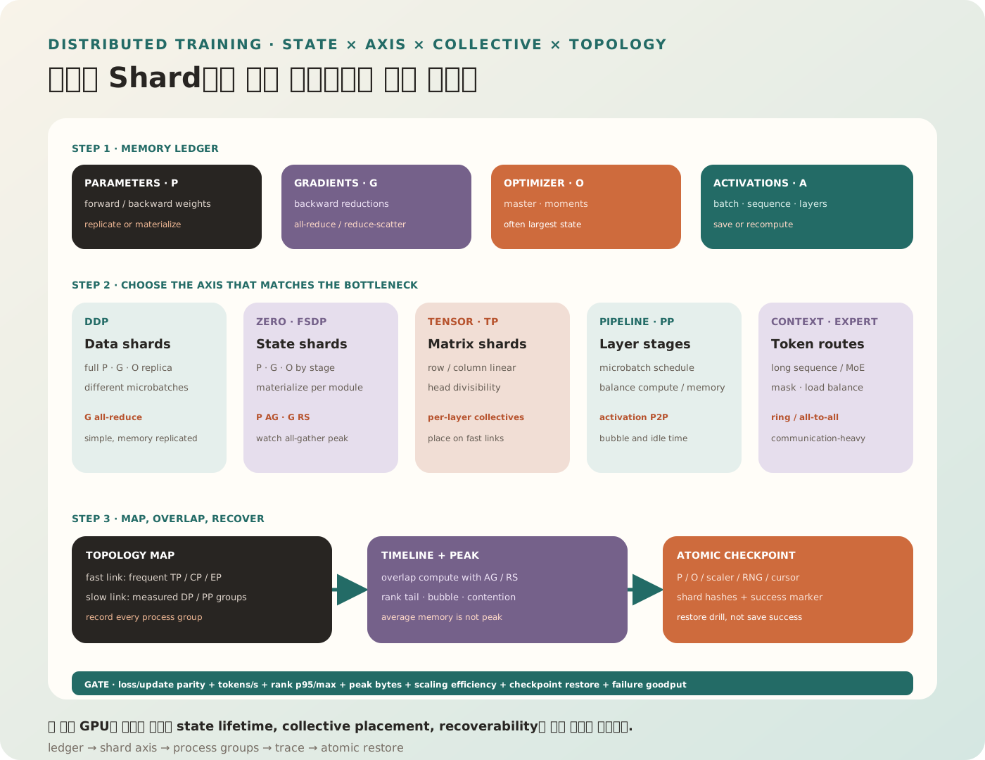

LLM 학습 memory 원장에서 parameter gradient optimizer activation을 분리하고 DDP, ZeRO FSDP, tensor, pipeline, context expert parallel의 shard와 collective를 topology, checkpoint, 성능 gate로 연결한 구조

그림 1. 각 parallelism은 다른 tensor 축과 state lifetime을 나눈다. Memory 절감만 보지 말고 collective의 위치, peak all-gather, bubble, 재시작 가능성을 함께 설계한다.

먼저 학습 Memory 원장을 만든다

분산 전략을 고르기 전에 한 step에서 무엇이 memory를 차지하는지 분리합니다.

training memory
  = parameters
  + gradients
  + optimizer states
  + activations
  + temporary buffers
  + allocator fragmentation

Parameter

Forward와 backward가 읽는 model weight입니다. BF16 또는 FP16이면 parameter 하나가 보통 2 byte지만, optimizer update를 위해 FP32 master weight를 별도로 둘 수 있습니다.

Gradient

각 trainable parameter에 대한 미분값입니다. Gradient dtype, accumulation 방식, unused parameter 처리에 따라 크기와 lifetime이 달라집니다.

Optimizer State

Adam 계열은 흔히 FP32 first moment m과 second moment v를 둡니다.

m ← β₁m + (1−β₁)g
v ← β₂v + (1−β₂)g²

Parameter 자체보다 optimizer state가 더 클 수 있습니다.

Activation

Backward에서 gradient를 계산하려고 forward 중간 결과를 보관합니다. Activation은 대략 다음 축에 따라 증가합니다.

microbatch × sequence length × hidden size × layers × saved tensors

Attention의 임시 tensor와 fused kernel 구현에 따라 단순 식보다 작거나 클 수 있습니다. Activation checkpointing을 쓰면 일부 activation을 저장하지 않고 backward 때 다시 계산합니다.

Temporary Buffer와 Peak

Collective bucket, fused optimizer workspace, attention workspace, parameter all-gather buffer가 있습니다. 평균 사용량이 device 용량보다 작아도 짧은 peak에서 OOM이 날 수 있습니다.

“Parameter당 16 byte”는 조건부 예시다

Mixed-precision Adam의 한 가지 예를 적어 봅니다.

항목	예시 dtype	Parameter당 byte
Forward parameter	BF16	2
Gradient	BF16	2
FP32 master parameter	FP32	4
Adam first moment	FP32	4
Adam second moment	FP32	4
합계		16

따라서 P개 parameter에 대해 model state만 대략 16P byte라는 계산이 나옵니다. 하지만 이것은 보편 상수가 아닙니다.

Master weight를 두지 않는 optimizer가 있습니다.
Gradient가 FP32일 수 있습니다.
8-bit optimizer state를 쓸 수 있습니다.
Frozen parameter와 trainable adapter의 상태가 다릅니다.
Padding, alignment, metadata, flat parameter가 추가됩니다.
Activation과 temporary peak는 이 계산에 없습니다.

Recipe를 먼저 쓰고 byte를 계산해야 합니다.

Global Batch를 Token으로 확인한다

DDP rank마다 다른 microbatch를 처리하고 gradient accumulation을 한다면 대략:

global sequences per update
  = microbatch_per_rank
  × gradient_accumulation_steps
  × data_parallel_world_size

고정 길이 padding이 많다면 sequence 수보다 유효 token 수가 더 정확합니다.

effective tokens per update
  = Σ non_padding_tokens over all ranks and accumulation steps

World size를 늘리면서 accumulation을 그대로 두면 global batch가 커집니다. Learning rate, warmup, optimizer dynamics가 달라질 수 있으므로 “GPU만 추가한 동일 실험”이 아닙니다.

Data Parallel: 계산 입력을 나눈다

DDP의 기본 동작

Distributed Data Parallel에서는 rank마다 model replica를 하나씩 둡니다.

rank 0: full model + batch shard 0
rank 1: full model + batch shard 1
rank 2: full model + batch shard 2
rank 3: full model + batch shard 3

각 rank가 forward와 backward를 수행한 뒤 gradient를 합칩니다. 대표적인 구현은 gradient bucket이 준비되는 대로 all-reduce를 시작해 남은 backward 계산과 겹칩니다.

local gradient gᵣ
all-reduce SUM(gᵣ)
divide by world size  # framework reduction convention 확인
same optimizer update on every rank

모든 rank가 동일한 초기 parameter와 동일한 reduced gradient로 update하면 replica가 동기화됩니다.

DDP가 잘 맞는 경우

Model과 optimizer state가 GPU 한 장에 충분히 들어갑니다.
Batch를 나누면 GPU별 계산량이 충분합니다.
Network가 gradient all-reduce를 감당합니다.
단순한 운영과 높은 compute utilization이 우선입니다.

DDP의 한계

Replica마다 parameter, gradient, optimizer state를 모두 보관하므로 model-state memory가 world size와 함께 줄지 않습니다. GPU를 늘려도 한 rank의 model memory는 거의 그대로입니다.

Distributed Sampler의 함정

모든 rank가 같은 sample을 읽으면 계산량만 늘고 effective batch diversity는 늘지 않습니다.

Epoch마다 sampler seed를 갱신합니다.
Drop-last와 padding sample 정책을 기록합니다.
Variable length packing 후 rank별 token 수를 관찰합니다.
Streaming data라면 rank와 worker별 shard가 겹치지 않는지 확인합니다.

Collective를 읽는 최소 어휘

All-reduce

모든 rank의 값을 합치고 결과를 모든 rank가 받습니다. DDP gradient 동기화의 대표 연산입니다.

All-gather

각 rank의 shard를 모아 모든 rank가 전체 값을 갖게 합니다. FSDP parameter materialization에서 사용됩니다.

Reduce-scatter

값을 합친 뒤 결과 shard를 rank별로 나눕니다. Sharded gradient 처리에 유용합니다.

All-to-all

각 rank가 서로 다른 조각을 모든 다른 rank에 보냅니다. Context parallel이나 expert parallel의 token 재배치에서 자주 나타납니다.

Point-to-point Send/Receive

Pipeline stage 사이 activation과 gradient를 넘길 때 사용합니다.

Collective 이름만으로 비용이 정해지지는 않습니다. Tensor byte, rank 수, topology, algorithm, contention, overlap이 함께 결정합니다.

ZeRO: 복제된 Model State를 단계별로 Shard한다

ZeRO는 data-parallel rank에 중복된 state를 나눕니다.

단계	Shard하는 상태	여전히 주로 복제되는 상태
ZeRO-1	Optimizer state	Parameter, gradient
ZeRO-2	Optimizer state, gradient	Parameter
ZeRO-3	Optimizer state, gradient, parameter	계산 시 필요한 parameter가 일시적으로 materialize

개념적 model-state memory는 DP rank 수 N에 따라 줄지만 정확한 peak는 bucket, padding, prefetch, persistence policy에 좌우됩니다.

ZeRO-1

각 rank가 optimizer state 일부만 소유하고 update한 parameter 조각을 동기화합니다. Optimizer state가 큰 Adam 계열에서 첫 memory 절감이 큽니다.

ZeRO-2

Gradient도 owner rank로 reduce-scatter합니다. 각 rank가 전체 gradient를 오래 보관할 필요가 줄어듭니다.

ZeRO-3

Parameter까지 shard합니다. Layer 계산 직전에 필요한 parameter shard를 all-gather하고, 계산 후 다시 버리거나 shard 상태로 돌립니다.

before layer compute: all-gather parameter shards
forward/backward: use materialized parameter
after compute: reshard/free full parameter
gradient: reduce-scatter to owners
optimizer: update local shard

Memory가 줄어드는 대신 layer 경계마다 통신이 생기며, prefetch와 reshard 정책이 peak와 성능을 바꿉니다.

FSDP: Module 실행 수명에 맞춘 Sharding

PyTorch Fully Sharded Data Parallel은 wrapped module 단위로 parameter를 shard하고 필요한 시점에 materialize합니다. Stable documentation의 대표 sharding 전략을 개념적으로 읽으면:

FULL_SHARD: parameter·gradient·optimizer state를 shard합니다.
SHARD_GRAD_OP: gradient와 optimizer state를 shard하고 parameter의 reshard 시점이 다릅니다.
NO_SHARD: model state를 복제하는 DDP와 비슷한 형태입니다.
Hybrid sharding: node 내부에서는 full shard, node 사이에서는 replica group을 둘 수 있습니다.

정확한 API 이름과 semantics는 사용하는 PyTorch version 문서를 기준으로 고정합니다.

Wrap Granularity

너무 큰 unit을 한 번에 all-gather하면 peak parameter memory가 큽니다. 너무 작은 unit은 collective 호출이 잦아 latency overhead가 커집니다.

large wrap unit
  + fewer collectives
  − larger materialization peak

small wrap unit
  + smaller peak
  − more frequent collectives

Transformer block 단위 auto-wrap은 좋은 출발점이지만 model architecture와 network에 맞춰 profile합니다.

Prefetch와 Rate Limiting

다음 layer parameter를 미리 all-gather하면 통신을 계산과 겹칠 수 있습니다. 너무 앞서 가져오면 여러 full parameter가 동시에 살아 peak memory가 커집니다.

ZeRO-3와 FSDP는 “완전히 같은 제품”이 아니다

둘 다 parameter·gradient·optimizer state sharding이라는 핵심 아이디어를 공유하지만 runtime, wrapping, checkpoint API, offload, prefetch 구현이 다릅니다. “Stage 3와 비슷한 목표”라고 이해하되 config를 그대로 번역하지 않습니다.

Tensor Parallel: Matrix 연산 내부를 나눈다

Model 한 layer조차 GPU 한 장에 들어가지 않거나, 큰 matrix multiplication을 여러 GPU가 함께 계산해야 할 때 사용합니다.

Linear layer를 생각해 봅니다.

Y = XW
W shape = [d_in, d_out]

Column Parallel

Output dimension을 나눕니다.

W = [W₀ | W₁ | ... | Wₜ₋₁]
Yᵢ = XWᵢ
Y = concat(Y₀, Y₁, ...)

다음 연산이 partitioned output을 그대로 소비할 수 있으면 즉시 gather하지 않을 수 있습니다.

Row Parallel

Input dimension을 나눕니다.

X = [X₀ | X₁ | ...]
W = vertical shards [W₀; W₁; ...]
partial Yᵢ = XᵢWᵢ
Y = Σ partial Yᵢ

Partial output을 합치기 위한 reduction이 필요합니다. Transformer MLP와 attention projection을 column/row pair로 배치하면 불필요한 gather를 줄일 수 있습니다.

Tensor Parallel의 조건

Layer마다 collective가 발생하므로 높은 bandwidth와 낮은 latency link가 중요합니다.
Hidden size, attention head, KV head, MLP dimension이 TP degree로 나뉘는지 확인합니다.
GQA에서는 query head와 KV head의 분할 규칙이 다를 수 있습니다.
Randomness, dropout, initialization이 shard 간 일관되어야 합니다.
Checkpoint tensor layout이 TP degree 변경을 지원하는지 확인합니다.

통신이 잦아 보통 빠른 intra-node interconnect 안에 TP group을 둡니다.

Pipeline Parallel: Layer 묶음을 Stage로 나눈다

Transformer block을 순서대로 여러 stage에 배치합니다.

stage 0: embedding + blocks 0...7
stage 1: blocks 8...15
stage 2: blocks 16...23
stage 3: blocks 24...31 + LM head

Stage 사이에는 activation을 forward 방향으로, activation gradient를 backward 방향으로 보냅니다.

왜 Microbatch가 필요한가

Batch 전체를 stage 0이 끝낸 뒤 stage 1로 넘기면 다른 stage가 오래 쉽니다. Batch를 m개 microbatch로 잘라 pipeline을 채웁니다.

time →
stage 0: F0 F1 F2 F3 ... B3 B2 B1 B0
stage 1:    F0 F1 F2 ... B3 B2 B1
stage 2:       F0 F1 ... B3 B2

Schedule은 GPipe식 all-forward/all-backward, 1F1B, interleaved schedule 등으로 달라집니다.

Bubble의 직관

단순한 균등 stage, forward-only fill 관점의 근사로 pipeline degree p, microbatch 수 m일 때 bubble 비율을 다음처럼 설명할 수 있습니다.

bubble fraction ≈ (p − 1) / (m + p − 1)

실제 training schedule은 forward/backward 시간, communication, interleaving, virtual stage 때문에 달라집니다. 식의 가정을 함께 기록합니다.

Stage Balance

Step time은 가장 느린 stage에 맞춰집니다.

Embedding과 LM head memory가 큽니다.
Layer별 FLOP가 동일하지 않을 수 있습니다.
MoE layer는 token routing에 따라 변동합니다.
Stage 경계 activation byte가 다릅니다.

Layer 수를 똑같이 나누는 것이 항상 균형 배치는 아닙니다. Profiled time과 memory로 partition합니다.

Sequence Parallel과 Context Parallel을 구분한다

Framework마다 용어 범위가 조금 다르므로 config 이름보다 “어느 activation을 어느 구간에서 나누는지”를 기록합니다.

Sequence Parallel

Tensor-parallel region에서 layer normalization, dropout 같은 연산의 activation을 sequence 축으로 shard해 중복 activation memory를 줄이는 방식으로 자주 쓰입니다. Attention이나 linear 연산에 들어갈 때 필요한 layout으로 collective를 수행합니다.

Context Parallel

긴 sequence의 attention 계산 자체를 여러 rank에 나눕니다.

tokens [0.........................L)
rank 0 [0.....L/4)
rank 1 [L/4...L/2)
rank 2 [L/2...3L/4)
rank 3 [3L/4......L)

각 query가 causal history의 key/value를 볼 수 있도록 KV block을 ring으로 전달하거나, head/sequence layout을 all-to-all로 바꿀 수 있습니다. DeepSpeed Ulysses는 sequence partition과 attention head partition 사이 all-to-all을 사용하는 대표 접근입니다.

긴 Context가 곧 쉬운 Scaling은 아니다

Attention mask와 position encoding이 partition 후에도 동일해야 합니다.
Load가 causal triangle 때문에 불균형할 수 있습니다.
Sequence length가 parallel degree로 잘 나뉘지 않을 수 있습니다.
KV communication byte와 compute overlap을 측정해야 합니다.
Packed sample 경계가 attention을 넘지 않도록 mask를 검증합니다.

Expert Parallel: MoE의 Expert를 나눈다

Mixture-of-Experts에서는 expert weight를 rank별로 배치하고 router가 선택한 token을 all-to-all로 보냅니다.

tokens
  → router top-k
  → all-to-all dispatch
  → local experts
  → all-to-all combine

평균 FLOP는 줄어도 특정 expert에 token이 몰리면 capacity overflow와 straggler가 생깁니다.

Router auxiliary loss와 load balance를 관찰합니다.
Expert capacity와 dropped-token policy를 기록합니다.
EP group을 빠른 network에 배치합니다.
Data parallel과 expert data parallel의 group 정의를 구분합니다.

여러 Parallel 축을 조합한다

대형 학습은 data, tensor, pipeline, context, expert 축을 함께 쓸 수 있습니다.

example logical mesh
  DP = 8
  TP = 4
  PP = 2
  CP = 2

independent axes라면 total GPUs = 8 × 4 × 2 × 2 = 128

Expert parallel은 다른 축과 group을 공유하거나 별도 mesh dimension일 수 있습니다. 모든 framework에서 단순히 DP × TP × PP × CP × EP라고 곱할 수 있는 것은 아닙니다. 실제 process-group diagram을 artifact로 남깁니다.

3D Parallelism

전통적으로 DP × TP × PP 조합을 3D parallelism이라 부릅니다.

TP가 layer 내부 matrix를 나눕니다.
PP가 layer depth를 나눕니다.
DP가 서로 다른 data를 처리합니다.

Context와 expert 축이 추가되면 더 높은 차원의 mesh가 됩니다.

Topology-aware Placement

예를 들어 node당 GPU 8장, node 사이 network가 상대적으로 느리다면:

within node: TP group 4 × CP/EP group 2
across nodes: DP replicas or PP links

이는 절대 규칙이 아닙니다. Collective byte와 빈도를 측정해 mapping합니다.

Hardware topology를 수집합니다.
Parallel axis별 collective와 tensor size를 적습니다.
가장 빈번하고 latency-sensitive한 통신을 빠른 link에 둡니다.
Cross-traffic이 겹치는지 profile합니다.
Node 장애 단위와 checkpoint 복구 단위도 고려합니다.

Process Group을 명시적으로 그린다

Rank 0 하나가 속한 group 예시는:

global rank 0
  data-parallel group:    [0, 8, 16, 24]
  tensor-parallel group:  [0, 1, 2, 3]
  pipeline group:         [0, 4]
  context-parallel group: [0, 32]

숫자는 예시입니다. Group 순서가 잘못되면 collective deadlock이나 잘못된 gradient reduction이 생깁니다. Config에서 추론하지 말고 시작 시 rank mapping을 log와 manifest에 남깁니다.

Activation Checkpointing: Memory를 계산으로 바꾼다

Checkpointing 구간의 input만 저장하고 내부 activation은 backward 때 forward를 다시 실행해 만듭니다.

without checkpointing:
  save a₁, a₂, a₃, a₄

with checkpointing:
  save boundary a₀
  backward time: recompute a₁...a₄

Trade-off

Activation memory가 줄어듭니다.
Forward compute 일부를 반복합니다.
RNG state를 올바르게 복구해야 dropout gradient가 일치합니다.
Communication도 다시 실행되는 구간인지 framework semantics를 확인합니다.
너무 작은 checkpoint unit은 overhead가 커집니다.

FSDP parameter all-gather와 activation recompute가 겹치면 예상보다 통신이 늘 수 있으므로 trace로 확인합니다.

CPU·NVMe Offload

Parameter나 optimizer state를 host memory 또는 storage로 옮기면 GPU memory는 줄지만 PCIe·network·storage bandwidth가 병목이 됩니다.

saved GPU bytes
  ↔ transfer bytes per step
  ↔ transfer latency
  ↔ host memory pressure

“들어간다”와 “충분한 속도로 학습된다”를 분리합니다. Page fault, pinned memory, NUMA placement, storage queue를 관찰합니다.

Mixed Precision과 Distributed Numerical Safety

Forward dtype과 accumulation dtype을 구분합니다.
FP16 loss scaling 상태를 checkpoint합니다.
Global gradient norm은 shard 전체를 대상으로 계산합니다.
Gradient clipping이 reduction 전인지 후인지 확인합니다.
한 rank의 NaN을 모든 rank가 빠르게 감지하도록 collective health check를 둡니다.
BF16 지원 hardware와 kernel fallback을 확인합니다.

Shard별 local norm만 clip하면 full-model norm clipping과 다른 update가 됩니다.

Step Timeline으로 Overlap을 확인한다

좋은 config는 이름이 아니라 timeline으로 판별합니다.

time →
compute:   [F L0][F L1][F L2][B L2][B L1][B L0]
param AG:          [AG L2]       [AG L1][AG L0]
grad RS:                         [RS L2][RS L1][RS L0]
idle:       ... gaps caused by dependency or network contention ...

AG는 all-gather, RS는 reduce-scatter입니다.

다음 질문을 trace에서 답합니다.

Collective가 compute 뒤에 직렬로 서 있는가?
Prefetch가 너무 빨라 memory peak를 만드는가?
여러 parallel group의 collective가 같은 link에서 충돌하는가?
한 rank만 data loading이나 kernel에서 느린가?
Allocator가 full parameter를 제때 반환하는가?

성능 지표

Step Time

Synchronous training에서는 가장 느린 rank가 step을 결정합니다.

step_time ≈ max(rank_step_time)

평균만 보면 straggler를 놓칩니다. Rank별 p50·p95·max를 봅니다.

Throughput

tokens_per_second = effective_nonpadding_tokens / step_time

Sample/sec는 sequence length가 달라지면 비교가 왜곡됩니다.

Model FLOPs Utilization

유효 model FLOP를 hardware theoretical peak와 비교한 근사 지표입니다. 어떤 FLOP 공식을 썼는지와 recomputation 포함 여부를 명시합니다.

Scaling Efficiency

Baseline n₀ GPU의 throughput을 T₀, n GPU throughput을 Tₙ이라 하면:

scaling_efficiency
  = Tₙ / (T₀ × n/n₀)

Strong Scaling과 Weak Scaling

Strong scaling: global workload를 고정하고 GPU를 늘립니다.
Weak scaling: GPU당 workload를 고정해 global workload도 늘립니다.

둘을 섞어 “선형 확장”이라고 보고하지 않습니다.

Goodput

유효한 학습 progress에 기여한 처리량입니다.

goodput
  = processed tokens
  − replayed tokens after failure
  − invalid/corrupt batches
  − work discarded by overflow or restart

정확한 정의는 팀이 합의합니다. Raw throughput이 높아도 잦은 장애와 재시작으로 goodput은 낮을 수 있습니다.

Sharded Checkpoint는 파일 묶음이 아니라 Protocol이다

분산 checkpoint는 다음 상태를 포함해야 합니다.

Model parameter shard와 layout metadata
Optimizer state shard
Learning-rate scheduler state
Mixed-precision scaler state
Random number generator state: Python, CPU, accelerator, model-parallel RNG
Global step, consumed sample/token 수
Data loader·stream cursor와 shuffle state
Parallel mesh와 world size
Model, tokenizer, optimizer, training config version
Source data manifest와 code commit

Atomic Commit

모든 rank가 각자 파일을 쓴 직후 “checkpoint 완료”라고 표시하면 안 됩니다.

1. write to checkpoint-step-1000.tmp/
2. every rank reports shard hash and success
3. coordinator validates manifest completeness
4. publish SUCCESS marker or atomic rename
5. retention process may delete older complete checkpoints

Incomplete directory에는 success marker가 없어야 합니다.

World-size 변경 복구

좋은 checkpoint system은 가능한 경우 저장한 shard를 logical full state로 해석해 새 world size에 repartition합니다.

saved: DP 16 × TP 4
resume: DP 8 × TP 8

모든 optimizer와 tensor layout이 자유로운 reshard를 지원하는 것은 아닙니다. 지원 matrix를 실제 restore test로 검증합니다.

Checkpoint 테스트는 Save가 아니라 Restore다

다음 drill을 자동화합니다.

짧게 학습하고 checkpoint를 저장합니다.
모든 process를 종료합니다.
같은 topology로 복구해 다음 batch와 loss를 비교합니다.
지원한다면 다른 world size로 복구합니다.
한 shard를 누락·손상시켜 fail-closed인지 확인합니다.
Data cursor가 이미 소비한 sample을 과도하게 반복하지 않는지 확인합니다.

장애 형태와 진단

Collective Deadlock

Rank마다 collective 호출 순서나 tensor shape가 다르면 멈출 수 있습니다.

처방: Rank별 operation sequence, group id, tensor shape를 기록하고 timeout 후 stack과 flight recorder를 수집합니다.

한 Rank의 OOM

Variable-length batch, MoE routing, parameter prefetch로 특정 rank만 peak가 클 수 있습니다.

처방: Rank별 allocated/reserved/peak와 batch token 수를 함께 기록합니다.

Straggler

느린 data shard, thermal throttling, network retransmission, shared filesystem contention이 원인일 수 있습니다.

처방: Step을 data, compute, collective, optimizer, checkpoint 구간으로 나누고 rank별 tail을 비교합니다.

Silent Divergence

Shard reduction, loss normalization, padding mask, gradient clipping 오류로 실행은 되지만 학습이 달라질 수 있습니다.

처방: 작은 model·batch에서 single-device reference와 parameter update를 수치 비교합니다.

Checkpoint Storm

모든 rank가 동시에 shared storage에 큰 shard를 쓰면 학습과 다른 job이 느려집니다.

처방: 비동기 staging, bandwidth limit, stagger, dedicated checkpoint tier를 검토하고 durability window를 명시합니다.

Parallelism 선택 순서

1. 단일 GPU Baseline을 만든다

작은 model 또는 짧은 sequence로라도 loss, sample order, kernel, step breakdown을 검증합니다.

2. DDP로 Throughput을 확장한다

Model state가 한 장에 들어가면 가장 단순한 출발점입니다. Global batch가 변하지 않도록 accumulation을 조정합니다.

3. State Memory가 부족하면 Sharding을 추가한다

Optimizer가 병목이면 ZeRO-1, gradient까지 크면 ZeRO-2, parameter도 들어가지 않으면 FSDP full sharding 또는 ZeRO-3를 검토합니다. 이는 개념적 순서이며 framework가 제공하는 조합을 따릅니다.

4. 한 Layer가 크거나 Compute가 부족하면 TP를 추가한다

빠른 link 안에서 layer GEMM을 나눕니다. Divisibility와 kernel efficiency를 먼저 확인합니다.

5. Depth Memory를 더 나눠야 하면 PP를 추가한다

Stage balance와 충분한 microbatch를 확보합니다.

6. Long-context Activation과 Attention이 병목이면 CP를 추가한다

단순 activation memory 문제는 checkpointing과 sequence parallel로 해결될 수도 있습니다. Attention 자체의 context 축을 나눠야 하는지 구분합니다.

7. MoE라면 EP를 Topology에 맞춘다

Token all-to-all과 expert imbalance가 새로운 병목입니다.

예시: 70B급 Full Fine-tuning 설계 사고법

숫자는 특정 hardware 처방이 아니라 질문 순서를 보여 주는 예시입니다.

requirements
  model: dense decoder
  context: long
  optimizer: Adam-family
  target: full fine-tuning

questions
  1. exact bytes for P/G/O/A?
  2. which state cannot fit per rank?
  3. sequence activation peak after checkpointing?
  4. fastest intra-node group size?
  5. expected all-gather/reduce-scatter bytes?
  6. global token batch held constant?
  7. checkpoint reshard and recovery tested?

후보를 비교합니다.

후보	Memory 장점	주 통신/비용	핵심 검증
DDP	단순	Gradient all-reduce	Model state가 한 장에 들어가는가
FSDP full shard	P/G/O 분산	Layer별 AG·RS	All-gather peak와 overlap
FSDP + TP	State와 layer compute 분산	FSDP + layer collective	Group contention과 checkpoint layout
TP + PP + DP	Layer·depth·data 분산	TP collective + P2P + DP reduce	Stage bubble과 topology
위 조합 + CP	Long-context 분산	KV/attention collective	Context correctness와 communication

Config를 선택한 뒤 32 GPU부터 바로 시작하지 않습니다. 1→2→한 node→두 node 순으로 parity와 scaling을 확인하면 deadlock과 수치 오류의 원인을 좁히기 쉽습니다.

RAG Agent 학습과 연결하기

RAG agent용 SFT·preference data는 길이와 구조 편차가 큽니다.

긴 retrieved context가 activation과 attention memory를 키웁니다.
Tool trace는 짧은 sample과 긴 sample의 편차가 큽니다.
Packed sequence에서 서로 다른 episode가 attention으로 섞이면 label leakage가 생깁니다.
JSON·tool token의 loss normalization이 rank별 padding과 함께 달라질 수 있습니다.
Retrieval corpus snapshot과 training data manifest가 checkpoint에 연결돼야 합니다.

따라서 token-balanced batching, exact attention mask, loss denominator의 global reduction을 검증합니다.

local loss numerator = Σ valid_token_loss
local valid tokens   = Σ loss_mask

global mean loss
  = all_reduce(Σ loss numerator)
  / all_reduce(Σ valid tokens)

Rank별 mean을 다시 단순 평균하면 valid token 수가 다른 rank에 같은 가중치를 줘 잘못된 loss가 될 수 있습니다.

실행 Manifest 예시

run:
  id: rag-agent-sft-dist-v8
  code_commit: abc1234
  model_manifest: model-v7
  data_manifest: rag-tool-traces-v11
precision:
  parameters: bfloat16
  gradients: bfloat16
  optimizer_states: float32
parallelism:
  world_size: 64
  data_parallel: 8
  tensor_parallel: 4
  pipeline_parallel: 2
  context_parallel: 1
  fsdp:
    mode: full_shard
    wrap_unit: transformer_block
batch:
  microbatch_per_rank: 1
  gradient_accumulation: 16
  report_nonpadding_tokens: true
checkpoint:
  format: sharded
  atomic_success_marker: true
  save_rng: true
  save_data_cursor: true
  restore_tested_world_sizes: [64]
evaluation:
  reference_parity_run: single-device-small
  report_rank_tail_latency: true

값은 예시입니다. world_size와 parallel axis의 관계는 framework mesh 정의로 검증해야 하며, 서로 독립이 아닌 축을 억지로 곱하지 않습니다.

흔한 오해와 처방

1. GPU를 두 배로 늘리면 학습이 두 배 빠르다

Collective, bubble, data loader, straggler 때문에 scaling efficiency가 떨어집니다.

처방: Strong/weak scaling을 구분하고 token/sec와 rank별 tail을 측정합니다.

2. DDP가 Model Memory를 GPU 수만큼 줄인다

DDP는 model replica를 각 rank에 둡니다.

처방: Model state를 줄이려면 ZeRO/FSDP 등 sharding을 검토합니다.

3. FSDP를 켜면 OOM은 사라진다

All-gather parameter, activation, temporary buffer peak가 남습니다.

처방: Wrap granularity, prefetch, reshard, activation checkpointing을 함께 profile합니다.

4. ZeRO-3와 FSDP config는 일대일로 대응한다

목표는 유사하지만 runtime와 API semantics가 다릅니다.

처방: 사용 framework의 versioned documentation과 trace를 기준으로 설정합니다.

5. TP는 통신을 줄인다

Layer마다 collective가 생길 수 있습니다.

처방: Fast link 안에 group을 두고 GEMM 크기와 communication overlap을 benchmark합니다.

6. Pipeline Stage에 Layer 수만 같으면 균형이다

Embedding, head, MoE, activation byte가 다릅니다.

처방: Profiled compute·memory·P2P byte로 partition합니다.

7. Checkpoint Directory가 있으면 복구 가능하다

일부 shard나 RNG, data cursor가 빠질 수 있습니다.

처방: Atomic manifest와 정기 restore drill을 운영합니다.

8. 모든 Rank의 Mean Loss를 평균하면 Global Mean이다

Valid token 수가 다르면 잘못된 가중치가 됩니다.

처방: Numerator와 denominator를 각각 all-reduce합니다.

Production 체크리스트

스스로 확인하기

Mixed-precision Adam의 model-state byte를 parameter·gradient·master weight·moment로 나눠 계산할 수 있는가?
DDP가 gradient를 합쳐도 parameter memory가 줄지 않는 이유는 무엇인가?
ZeRO-1·2·3은 각각 어떤 state를 shard하는가?
FSDP wrap unit을 너무 크게 또는 작게 잡으면 어떤 문제가 생기는가?
Column parallel과 row parallel linear에서 어떤 collective가 필요한가?
Pipeline bubble을 줄이기 위해 microbatch 수와 stage balance를 어떻게 조절하는가?
Sequence parallel과 context parallel을 tensor lifetime 관점에서 구분할 수 있는가?
Rank별 valid token 수가 다를 때 global mean loss를 어떻게 계산하는가?
Sharded checkpoint의 success marker를 모든 shard 검증 뒤에 써야 하는 이유는 무엇인가?
Throughput과 goodput이 달라지는 장애 시나리오를 설명할 수 있는가?

앞 글에서 model representation을 줄이는 법을, 이 글에서 학습 state와 compute를 여러 device에 나누는 법을 연결했습니다. 다음 글은 효율적인 LLM 추론 서빙: Prefill·Decode·KV Cache·Batching입니다. 학습용 parallelism과 serving용 scheduling이 왜 다른지 TTFT·ITL·throughput·SLO로 분석합니다.