Field Log · Entry

현대 Decoder LLM 구조: RMSNorm·RoPE·GQA·SwiGLU·MoE (3/10)

Residual stream이 pre-RMSNorm, RoPE와 GQA attention, SwiGLU 또는 routed MoE를 통과하며 KV cache와 token compute를 결정하는 decoder block

오늘의 결론

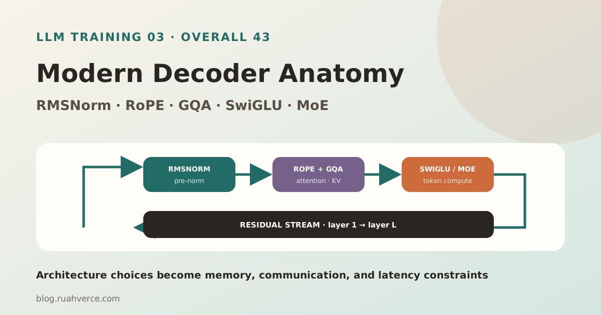
현대 decoder-only LLM은 Transformer 원형을 유지하면서 pre-norm, RMSNorm, RoPE, SwiGLU, GQA 같은 선택을 조합합니다.

Residual stream은 정보와 gradient가 흐르는 주 경로이고, pre-norm은 attention·FFN sublayer에 들어가기 전에 activation을 정규화합니다.

GQA는 query head 수가 아니라 key/value head 수를 줄여 decode의 KV cache와 memory bandwidth 부담을 낮춥니다.

SwiGLU는 FFN에 gate를 추가합니다. MoE는 FFN을 여러 expert로 바꾸고 token마다 일부만 활성화해 total parameter와 active compute를 분리합니다.

Architecture config의 작은 차이는 checkpoint 호환성, kernel, parallelism, memory, latency까지 바꾸므로 이름이 아니라 tensor shape를 읽어야 합니다.

앞 글에서는 model parameter N, token D, compute C를 배분했습니다. 이제 그 parameter가 decoder block 안에서 무엇을 하는지 봅니다.

token IDs
  → embeddings
  → decoder block × L
  → final norm
  → vocabulary logits
  → next-token probability

“Transformer를 안다”와 “어떤 LLM checkpoint가 왜 빠르고 느린지 설명한다” 사이에는 구조 세부가 있습니다.

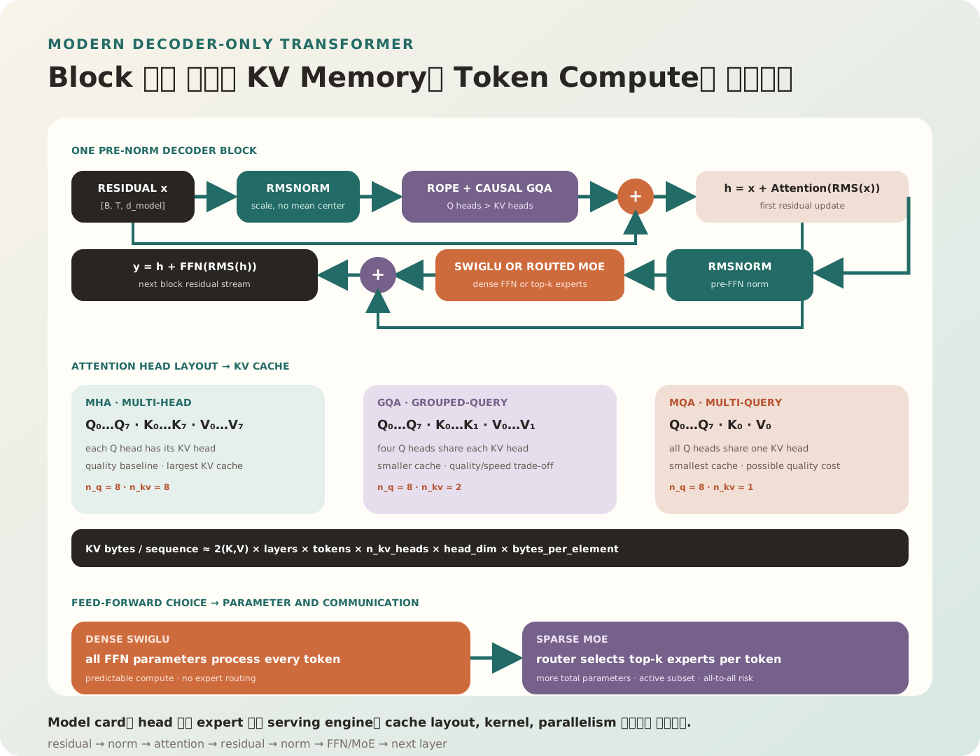
Residual stream이 pre-RMSNorm과 RoPE GQA attention, 다시 RMSNorm과 dense SwiGLU 또는 routed MoE를 통과하고 KV head와 expert 수가 serving 비용을 만드는 구조

그림 1. 한 block의 수식만 보지 말고 attention head layout이 KV cache로, FFN 방식이 parameter·communication 비용으로 이어지는 경로를 함께 본다.

먼저 Tensor Shape를 읽자

일반적인 decoder config를 기호로 둡니다.

B       batch size
T       sequence length
d       hidden size = d_model
L       number of decoder layers
n_q     number of query heads
n_kv    number of key/value heads
d_h     head dimension
d_ff    feed-forward intermediate size
V       vocabulary size

보통 다음 관계가 있습니다.

d = n_q × d_h

Hidden state shape는 다음과 같습니다.

X ∈ R[B, T, d]

Model config를 읽을 때 parameter 이름보다 shape를 먼저 확인하면 MHA, GQA, MQA와 FFN 크기를 계산할 수 있습니다.

Decoder-only라는 뜻

원래 Transformer는 encoder와 decoder를 함께 사용했습니다. 많은 생성형 LLM은 causal self-attention을 쌓은 decoder-only 구조입니다.

encoder-decoder
  source → bidirectional encoder
  target → causal decoder + cross attention

decoder-only
  one token stream → causal self-attention

Prompt, retrieved context, tool result, assistant output을 한 token sequence에 직렬화하고 causal mask로 다음 token을 예측합니다.

Residual Stream이 주 경로다

Sublayer가 만든 변화량을 입력에 더합니다.

h = x + Attention(Norm(x))
y = h + FFN(Norm(h))

x → h → y가 residual stream입니다.

왜 더하는가

초기에는 sublayer가 작은 수정만 학습할 수 있습니다.
깊은 network에서 identity path가 유지됩니다.
Gradient가 sublayer 외의 짧은 경로로도 흐릅니다.
각 layer가 representation 전체를 매번 다시 만들 필요가 없습니다.

Residual add를 할 때 tensor shape는 같아야 합니다.

Attention output: [B, T, d]
FFN output:       [B, T, d]
Residual:         [B, T, d]

Post-norm과 Pre-norm

Post-norm

원래 Transformer 식은 sublayer 뒤에 normalization을 적용하는 형태로 알려져 있습니다.

h = Norm(x + Attention(x))
y = Norm(h + FFN(h))

Pre-norm

많은 현대 LLM은 sublayer 전에 normalization을 둡니다.

h = x + Attention(Norm(x))
y = h + FFN(Norm(h))

Pre-norm은 residual identity path를 normalization 밖에 두어 깊은 network의 optimization을 안정화하는 데 자주 사용됩니다.

어느 쪽이 무조건 우수한가

아닙니다. Final quality, depth, initialization, learning rate, residual scaling에 따라 다릅니다. 체크포인트가 어떤 ordering으로 학습되었는지는 weight만 보고 임의로 바꿀 수 없습니다.

LayerNorm과 RMSNorm

LayerNorm

한 token의 hidden vector x ∈ R^d에 대해 평균과 분산을 사용합니다.

μ = (1/d) Σᵢ xᵢ
σ² = (1/d) Σᵢ (xᵢ − μ)²

LayerNorm(x)ᵢ
= γᵢ (xᵢ − μ) / sqrt(σ² + ε) + βᵢ

RMSNorm

RMSNorm은 mean centering을 생략하고 root mean square로 scale을 정규화합니다.

rms(x) = sqrt((1/d) Σᵢ xᵢ² + ε)

RMSNorm(x)ᵢ
= γᵢ xᵢ / rms(x)

원 논문은 LayerNorm의 re-centering invariance가 필수적이지 않을 수 있다는 가설에서 RMSNorm을 제안했습니다.

“RMSNorm은 항상 더 빠르다”가 아닌 이유

연산 정의는 단순하지만 end-to-end 속도는 다음에 달려 있습니다.

fused kernel 존재
hidden size와 batch shape
memory access
dtype
compiler와 serving engine
다른 kernel과 fusion 가능성

Model architecture 수준의 연산 감소와 실제 latency를 구분합니다.

ε도 Config다

{
  "rms_norm_eps": 1e-5
}

Checkpoint를 다른 epsilon으로 load하면 동일 model이 아닙니다. Dtype에 따른 numerical behavior도 확인합니다.

Attention을 Shape로 다시 보기

Input X를 query, key, value로 projection합니다.

Q = XW_Q
K = XW_K
V = XW_V

한 head의 scaled dot-product attention은 다음입니다.

Attention(Q, K, V)
= softmax((QKᵀ / sqrt(d_h)) + causal_mask) V

Query는 “찾고 싶은 것”

현재 position이 과거 token에서 어떤 정보를 가져올지 표현합니다.

Key는 “매칭 주소”

각 과거 position이 어떤 query와 관련 있는지 비교하는 표현입니다.

Value는 “가져올 내용”

Attention probability로 가중 합할 내용 표현입니다.

이 비유는 직관일 뿐, 학습된 vector에 사람이 정한 고정 의미가 들어 있다는 뜻은 아닙니다.

Multi-Head Attention

MHA에서는 각 query head가 자신만의 key와 value head를 가집니다.

n_q = n_kv

Q: [B, n_q,  T, d_h]
K: [B, n_kv, T, d_h]
V: [B, n_kv, T, d_h]

여러 head가 서로 다른 relation pattern을 학습할 capacity를 제공합니다.

Projection Parameter 근사

Bias를 생략하면 MHA의 QKV와 output projection은 대략 다음과 같습니다.

W_Q: d × d
W_K: d × d
W_V: d × d
W_O: d × d

total ≈ 4d²

MQA: Key와 Value를 하나만 공유한다

Multi-Query Attention에서는 query head는 여러 개지만 KV head는 하나입니다.

n_q > 1
n_kv = 1

모든 query head가 같은 K와 V를 공유합니다.

장점은 decode에서 KV cache 크기와 읽기 bandwidth를 크게 줄일 수 있다는 점입니다. 다만 공유가 강해져 quality trade-off가 생길 수 있습니다.

GQA: 중간 지점

Grouped-Query Attention은 query head를 group으로 묶고 group마다 KV head 하나를 공유합니다.

n_q = 32
n_kv = 8
group_size = n_q / n_kv = 4

Query head 4개가 KV head 하나를 공유합니다.

GQA 논문은 기존 multi-head checkpoint를 grouped-query model로 uptrain하는 방법과 MHA 품질에 가깝고 MQA 속도에 가까운 trade-off를 연구했습니다. 이 결과는 논문 실험 조건이며 모든 model에 동일한 차이를 보장하지 않습니다.

GQA Tensor Shape

Q: [B, 32, T, d_h]
K: [B,  8, T, d_h]
V: [B,  8, T, d_h]

Attention 계산 시 KV head가 대응하는 query group에 broadcast 또는 repeat되는 논리 구조를 가집니다. 실제 kernel은 물리적으로 불필요한 복사를 피해야 합니다.

KV Cache가 구조 선택을 비용으로 바꾼다

Autoregressive decode에서 이전 token의 K와 V를 매 step 다시 계산하지 않고 저장합니다.

한 sequence의 KV cache byte를 단순 근사하면 다음과 같습니다.

KV_bytes
≈ 2
 × L
 × T
 × n_kv
 × d_h
 × bytes_per_element

2: K와 V
L: layer 수
T: cache된 token 수
n_kv: KV head 수
d_h: head dimension

Allocator metadata, alignment, quantization scale, prefix sharing 같은 실제 overhead·절감은 제외한 식입니다.

가상 계산

L = 32
T = 8192
d_h = 128
dtype = BF16 = 2 bytes

MHA n_kv = 32:

2 × 32 × 8192 × 32 × 128 × 2
= 4,294,967,296 bytes
≈ 4 GiB per sequence

GQA n_kv = 8:

≈ 1 GiB per sequence

MQA n_kv = 1:

≈ 128 MiB per sequence

가상 config의 근사치입니다. 하지만 n_kv가 long-context 동시성에 얼마나 큰 영향을 주는지 보여 줍니다.

Prefill과 Decode에서 Attention 병목이 다르다

Prefill

Prompt 전체 token을 병렬 처리합니다.

Q: many prompt positions
K,V: many prompt positions
attention matrix: T × T

긴 context에서는 attention 계산과 memory I/O가 큽니다.

Decode

새 token 하나를 생성합니다.

Q: one new position
K,V: all cached positions

매 step cache를 읽으므로 memory bandwidth와 KV 크기가 중요합니다. GQA가 serving에서 특히 가치 있는 이유입니다.

Position 정보가 필요한 이유

Attention의 dot product 자체는 token 순서가 바뀌어도 같은 set을 볼 수 있습니다. Sequence order를 표현할 position mechanism이 필요합니다.

Learned Absolute Position

각 position index의 embedding을 token embedding에 더할 수 있습니다.

h₀ = token_embedding + position_embedding

학습한 최대 position 바깥으로 확장하는 문제가 있습니다.

RoPE

Rotary Position Embedding은 query와 key vector의 2차원 성분 쌍을 position에 따라 회전시킵니다.

단순 2D 쌍 (a, b)에 각도 θ_t를 적용하면 다음과 같습니다.

[a']   [ cos θ_t  −sin θ_t ] [a]
[b'] = [ sin θ_t   cos θ_t ] [b]

Query와 key에 position-dependent rotation을 적용하면 attention dot product에 relative position 차이가 반영됩니다.

q_t' = R_t q_t
k_s' = R_s k_s

q_t'ᵀ k_s'
= q_tᵀ R_(s−t) k_s

표현을 단순화한 식이지만 relative offset이 들어오는 핵심을 보여 줍니다.

RoPE Config를 읽는 법

{
  "rope_theta": 10000,
  "max_position_embeddings": 8192,
  "rope_scaling": null
}

확인할 항목은 다음과 같습니다.

base 또는 theta
rotary를 적용하는 head dimension 비율
original training context
scaling method와 factor
position ID 처리
cache 재사용 시 position offset

Context Window를 숫자 하나로 늘리면 안 된다

Config의 max_position_embeddings만 바꿔도 model이 긴 context를 이해하게 되는 것은 아닙니다.

학습 distribution 밖의 position
high/low-frequency rotation behavior
long-context fine-tuning 필요
attention sink와 lost-in-the-middle
KV cache memory
kernel 지원 범위
evaluation contamination

RoPE scaling 기법은 별도의 가정과 trade-off가 있으므로 model card와 학습 recipe를 따라야 합니다.

FFN은 Token별 비선형 변환이다

Attention이 position 사이 정보를 섞는다면 FFN은 각 position에 같은 network를 독립 적용합니다.

원형은 다음과 같습니다.

FFN(x) = W_down activation(W_up x)

Shape는 대략 다음입니다.

W_up:   d → d_ff
W_down: d_ff → d

FFN parameter는 layer parameter의 큰 비중을 차지할 수 있습니다.

GLU와 SwiGLU

Gated Linear Unit 계열은 두 projection의 element-wise product를 사용합니다.

SwiGLU를 단순화하면 다음과 같습니다.

gate = SiLU(xW_gate)
up   = xW_up

SwiGLU(x)
= (gate ⊙ up) W_down

여기서 SiLU 또는 swish는 다음과 같습니다.

SiLU(z) = z × sigmoid(z)

세 Matrix가 있다

W_gate: d × d_ff
W_up:   d × d_ff
W_down: d_ff × d

Parameter는 bias를 빼면 대략 3dd_ff입니다.

같은 parameter budget에서 ReLU/GELU FFN과 비교하려면 d_ff를 조정할 수 있습니다. 단순히 intermediate size 숫자만 비교하면 안 됩니다.

Gate의 직관

up branch가 만든 feature를 gate branch가 position·feature별로 조절합니다. “어떤 knowledge neuron을 켠다”처럼 너무 문자 그대로 해석하지는 않습니다.

GLU Variants 논문은 Transformer FFN에서 여러 gated activation을 비교해 일부 variant의 quality 개선을 보고했습니다. 그 결과가 모든 architecture와 budget에서 자동으로 재현된다는 뜻은 아닙니다.

Dense FFN과 MoE

Dense

모든 token이 같은 FFN parameter를 통과합니다.

token → one shared FFN → output

Total parameter와 token당 active parameter가 같습니다.

Mixture-of-Experts

FFN을 여러 expert로 두고 router가 token마다 일부 expert를 선택합니다.

router scores = softmax(xW_router)
selected = top_k(router scores)

MoE(x)
= Σ_{e ∈ selected} g_e(x) Expert_e(x)

Total과 Active Parameter

8 experts
top-2 routing

total expert parameters: 8 × one_expert
active per token:         2 × one_expert

Attention과 embedding 같은 shared parameter는 별도로 항상 활성화됩니다.

Mixtral 사례를 읽는 법

Mixtral of Experts 논문은 각 layer의 feed-forward block에 8개 expert를 두고 token마다 2개를 선택하는 sparse MoE를 설명합니다.

이를 “47B model인데 13B처럼 계산한다” 같은 한 문장으로만 외우면 안 됩니다.

Total checkpoint memory는 전체 expert를 저장합니다.
Token compute는 selected expert와 shared layers를 포함합니다.
Batch의 token이 여러 expert로 흩어지면 다수 expert가 동시에 활성화됩니다.
Multi-GPU에서는 token dispatch와 combine 통신이 필요합니다.
Expert load imbalance가 utilization을 떨어뜨릴 수 있습니다.

Router가 만드는 새 문제

Load Imbalance

특정 expert에 token이 몰릴 수 있습니다.

expert 0: 42% tokens
expert 1: 18%
expert 2:  9%
...

가장 바쁜 expert 때문에 step이 느려집니다.

Capacity

Expert가 한 batch에서 받을 token 수에 capacity limit를 둘 수 있습니다.

Limit를 넘은 token을 drop, reroute, pad하는 정책은 architecture와 implementation에 따라 다릅니다.

Auxiliary Load-balancing Loss

Router가 expert를 고르게 쓰도록 보조 loss를 둘 수 있습니다. 가중치가 너무 크면 task loss와 충돌하고, 너무 작으면 imbalance가 남습니다.

Expert Parallel Communication

tokens on GPU A
  → all-to-all dispatch
  → experts on GPUs A/B/C/D
  → expert compute
  → all-to-all combine

Network topology와 message size가 성능을 좌우합니다.

MoE가 항상 더 빠른가

아닙니다.

작은 batch에서는 dispatch overhead가 큽니다.
모든 expert weight가 device memory에 맞지 않을 수 있습니다.
Expert parallel network가 느릴 수 있습니다.
Uneven routing으로 GPU가 놀 수 있습니다.
Serving request 간 token distribution이 불안정합니다.
Engine이 해당 MoE kernel을 최적화하지 않았을 수 있습니다.

동일 quality, hardware, batch, context에서 benchmark합니다.

Parameter Count를 직접 근사하기

Dense layer의 주요 parameter를 bias 없이 단순화합니다.

GQA Attention

Q projection: d × (n_q  × d_h) = d × d
K projection: d × (n_kv × d_h)
V projection: d × (n_kv × d_h)
O projection: d × d

따라서:

P_attention
≈ 2d² + 2d(n_kv d_h)

MHA에서 n_kv = n_q이면 ≈ 4d²가 됩니다.

SwiGLU FFN

P_ffn ≈ 3d d_ff

Layer 전체

P_layer
≈ P_attention + P_ffn + norm scales

Embedding과 output head, weight tying, final norm을 별도로 더합니다.

Config 예시를 해석하기

{
  "hidden_size": 4096,
  "num_hidden_layers": 32,
  "num_attention_heads": 32,
  "num_key_value_heads": 8,
  "intermediate_size": 11008,
  "hidden_act": "silu",
  "rms_norm_eps": 1e-5,
  "rope_theta": 10000,
  "vocab_size": 64000,
  "tie_word_embeddings": false
}

Head Dimension

d_h = hidden_size / num_attention_heads
    = 4096 / 32
    = 128

GQA Group Size

group_size = 32 / 8 = 4

KV Projection Width

n_kv × d_h = 8 × 128 = 1024

FFN Parameter per Layer

3 × 4096 × 11008
≈ 135.3M parameters

실제 checkpoint에는 implementation 세부, bias, tied weight, padding된 tensor가 있으므로 state dict로 검증합니다.

Weight Tying

Input embedding과 output vocabulary projection weight를 공유할 수 있습니다.

E ∈ R[V, d]

input:  token_id → E[token_id]
output: logits = h Eᵀ

tie_word_embeddings: true면 parameter와 memory를 줄일 수 있지만 모든 model이 사용하지 않습니다. Checkpoint conversion에서 두 tensor를 잘못 중복하거나 공유하면 file size와 결과가 달라집니다.

Logits와 Final Norm

마지막 layer 뒤에 final RMSNorm 또는 LayerNorm을 적용한 뒤 vocabulary logits를 만듭니다.

h_final = FinalNorm(h_L)
logits = h_final W_vocabᵀ
p = softmax(logits)

Training cross-entropy는 전체 vocabulary logits가 필요할 수 있고, inference sampling은 logits processor와 decoding policy를 추가합니다.

Architecture와 Checkpoint 호환성

다음 중 하나만 달라도 단순 reshape로 해결되지 않을 수 있습니다.

layer 수
hidden size
query/KV head 수
head dimension
RoPE convention
norm type와 epsilon
FFN activation과 intermediate size
MoE expert 수와 top-k
vocabulary와 special token ID
weight tying
QKV fused layout

QKV Layout 예

implementation A:
  separate q_proj, k_proj, v_proj

implementation B:
  fused qkv_proj

implementation C:
  head-interleaved packed tensor

Tensor element 수가 같아도 ordering이 다르면 conversion 후 출력이 망가집니다.

Conversion Verification

1. same tokenizer and prompt
2. same dtype or high-precision reference
3. compare layer-0 hidden states
4. compare selected intermediate layers
5. compare final logits
6. compare greedy token sequence

최종 text만 비교하면 작은 오차가 sampling에서 증폭되어 원인을 찾기 어렵습니다.

Architecture가 Quantization에 미치는 영향

뒤의 양자화 글에서 자세히 다루지만 구조를 먼저 연결해 둡니다.

RMSNorm scale과 activation outlier
Q/K projection precision과 attention error
GQA의 작은 KV tensor와 KV quantization
SwiGLU gate branch의 sensitivity
MoE expert별 calibration coverage
Router logits precision과 expert 선택 변화

MoE calibration data가 일부 expert를 거의 활성화하지 않으면 해당 expert weight의 quantization 품질을 검증하지 못합니다.

Architecture가 Parallelism에 미치는 영향

Tensor Parallel

Attention과 FFN matrix를 여러 device에 나눕니다. Head 수와 intermediate size가 parallel degree로 잘 나뉘는지 중요합니다.

n_q % tensor_parallel_degree == 0
n_kv compatibility must be checked
d_ff partition must be supported

GQA에서 n_kv가 TP degree보다 작으면 KV head replication 같은 engine별 처리가 필요할 수 있습니다.

Pipeline Parallel

Layer를 stage로 나눕니다. Layer별 parameter와 compute가 비슷한 dense model은 비교적 균등 분할하기 쉽지만 embedding/output head와 MoE layer는 imbalance를 만들 수 있습니다.

Expert Parallel

MoE expert를 device에 나눕니다. Router의 token distribution과 network topology가 새 축이 됩니다.

Architecture가 RAG Agent에 미치는 영향

Long Retrieved Context

Context length가 길수록 KV cache가 선형으로 증가합니다. GQA, cache quantization, prefix caching 지원을 확인합니다.

Multi-turn Agent

매 turn history와 tool result가 늘어납니다. 작은 n_kv는 동시 session 수를 늘리는 데 도움이 될 수 있습니다.

Tool Schema

Architecture만으로 structured output 능력이 결정되지는 않습니다. Tokenizer, SFT, preference training, constrained decoding이 함께 필요합니다.

Repeated Short Calls

Planner·router·verifier처럼 짧은 호출이 많으면 kernel launch와 scheduling overhead도 중요합니다. 큰 MoE의 이론 active parameter 이점이 작은 batch latency로 이어지는지 측정합니다.

Model Card에서 확인할 표

영역	확인 필드	운영 영향
hidden	layers, d_model, d_ff	weight·activation memory
attention	n_q, n_kv, d_h	KV cache·TP compatibility
position	RoPE theta, scaling, trained context	long-context validity
normalization	type, epsilon, ordering	checkpoint·kernel compatibility
FFN	activation, gate, bias	parameter·kernel
MoE	experts, top-k, capacity	memory·all-to-all·load balance
embedding	vocab, tying	weight memory·tokenizer match
precision	supported dtypes	kernel·accuracy

Benchmark Matrix

benchmark:
  hardware: fixed
  engine_version: fixed
  dtype: bf16
  cases:
    - prompt_tokens: 512
      output_tokens: 128
      concurrency: [1, 8, 32]
    - prompt_tokens: 8192
      output_tokens: 256
      concurrency: [1, 8]
    - prompt_tokens: 32768
      output_tokens: 128
      concurrency: [1, 4]
  report:
    - time_to_first_token
    - inter_token_latency
    - request_latency_p50_p95
    - prefill_tokens_per_second
    - decode_tokens_per_second
    - peak_weight_memory
    - peak_kv_memory
    - max_stable_concurrency

Model 이름만 바꿔 benchmark하지 말고 architecture와 serving engine의 최적화 지원을 같이 기록합니다.

흔한 오해와 처방

1. RMSNorm은 LayerNorm에서 평균만 뺀 사소한 차이다

정의와 checkpoint parameterization이 다릅니다.

처방: Norm type, ordering, epsilon, fused kernel을 config와 state dict에서 확인합니다.

2. RoPE면 무한 Context다

Position mechanism이 있다는 것과 학습 범위 밖 long-context 품질은 다릅니다.

처방: 학습 context, scaling recipe, long-context eval, KV memory를 함께 검증합니다.

3. GQA는 Attention Head를 줄인다

Query head는 유지하고 KV head를 group별 공유하는 구조입니다.

처방: num_attention_heads와 num_key_value_heads를 따로 읽습니다.

4. KV Cache는 Model Size에만 비례한다

Layer, context, KV head, head dimension, dtype, 동시 sequence에 비례합니다.

처방: target context와 concurrency로 직접 byte를 계산합니다.

5. SwiGLU는 Activation 이름 하나다

Gate와 up projection 두 branch, down projection까지 세 matrix가 있습니다.

처방: d_ff와 gate layout으로 parameter·kernel을 계산합니다.

6. MoE의 Total Parameter가 곧 Token Compute다

Token은 top-k expert만 통과하지만 shared layer와 communication 비용이 있습니다.

처방: total·active parameter, dispatch bytes, expert utilization을 분리합니다.

7. MoE는 항상 Dense보다 싸다

Small batch와 느린 interconnect에서는 routing overhead가 이점을 지울 수 있습니다.

처방: target traffic와 topology에서 latency·throughput을 측정합니다.

8. 같은 Shape면 Checkpoint를 변환할 수 있다

QKV ordering과 RoPE convention이 다를 수 있습니다.

처방: intermediate activation과 logits를 layer별 비교합니다.

Production 체크리스트

스스로 확인하기

Pre-norm decoder block의 두 residual 식을 직접 쓸 수 있는가?
RMSNorm과 LayerNorm의 계산 차이는 무엇인가?
n_q = 32, n_kv = 8인 GQA에서 query group 크기는 얼마인가?
KV cache byte가 어떤 다섯 변수에 비례하는가?
SwiGLU가 일반 two-matrix FFN보다 projection 하나를 더 갖는 이유는 무엇인가?
MoE에서 total parameter와 active parameter가 다른 이유는 무엇인가?
같은 model이라도 MoE serving이 network topology에 따라 달라지는 이유는 무엇인가?

앞 글에서 학습 예산을, 이 글에서 decoder 구조를 연결했습니다. 다음 글은 Instruction Tuning과 SFT입니다. Base model의 next-token 능력을 system·user·assistant 대화 형식, response-only loss mask, 고품질 instruction data로 “요청을 따르는 행동”으로 바꾸는 과정을 다룹니다.