Field Log · Entry

GPU Roofline으로 LLM 추론 병목 읽기: FLOPS·Bandwidth·Arithmetic Intensity (1/10)

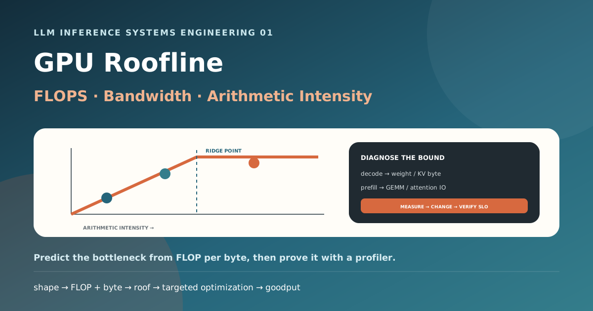
LLM prefill과 decode 연산을 arithmetic intensity와 GPU compute 및 memory bandwidth 지붕선 위에 배치해 병목과 최적화 방향을 찾는 구조

오늘의 결론

GPU가 바쁘다는 사실만으로는 병목을 알 수 없습니다. 초당 연산량과 초당 이동 byte를 함께 재고, FLOP/byte인 arithmetic intensity로 연결해야 합니다.

Roofline의 기본 상한은 min(peak compute, memory bandwidth × arithmetic intensity)입니다. Ridge point 왼쪽은 bandwidth, 오른쪽은 compute가 먼저 제한합니다.

같은 Transformer layer도 긴 prompt를 한꺼번에 처리하는 prefill과 새 token 하나를 만드는 decode의 shape가 달라 병목이 달라집니다. Decode는 weight와 KV를 재사용할 batch가 작으면 memory-bound가 되기 쉽습니다.

Roofline은 kernel 상한을 설명하지만 queue, scheduler, CPU, network, collective, kernel launch stall을 자동으로 설명하지 않습니다. End-to-end trace와 함께 써야 합니다.

최적화는 이름이 아니라 제거할 병목으로 고릅니다. Bandwidth-bound라면 byte를 줄이거나 재사용하고, compute-bound라면 연산 kernel과 precision을 개선하며, launch·통신 병목이면 별도 모델이 필요합니다.

앞 시리즈 마지막 글에서는 요청마다 모델·검색·검증 경로를 골랐습니다. 이제 선택된 모델이 GPU에서 실행될 때 왜 느린지 수치로 내려갑니다. 효율적인 LLM 추론 서빙 전체 지도가 scheduler와 SLO의 큰 그림이었다면, 이번 10편은 각 층의 계산과 구현을 하나씩 분해합니다.

느리다
  → 어느 phase인가: queue / prefill / decode / stream?
  → 어느 resource인가: compute / HBM / launch / communication?
  → 이론 상한과 실제 achieved 값의 간격은 얼마인가?
  → byte·FLOP·batch·shape 중 무엇을 바꿀 것인가?
  → TTFT·TPOT·goodput이 실제로 좋아졌는가?

이 글에서 답하는 질문

FLOPS와 memory bandwidth는 왜 따로 보면 부족한가?
Arithmetic intensity와 ridge point를 어떻게 계산하는가?
Linear layer의 prefill과 decode가 다른 병목을 갖는 이유는 무엇인가?
Attention에서는 weight 외에 어떤 byte가 이동하는가?
Profiler 수치를 Roofline 위에 어떻게 놓는가?
Compute·bandwidth·launch·통신 병목마다 어떤 최적화를 선택하는가?

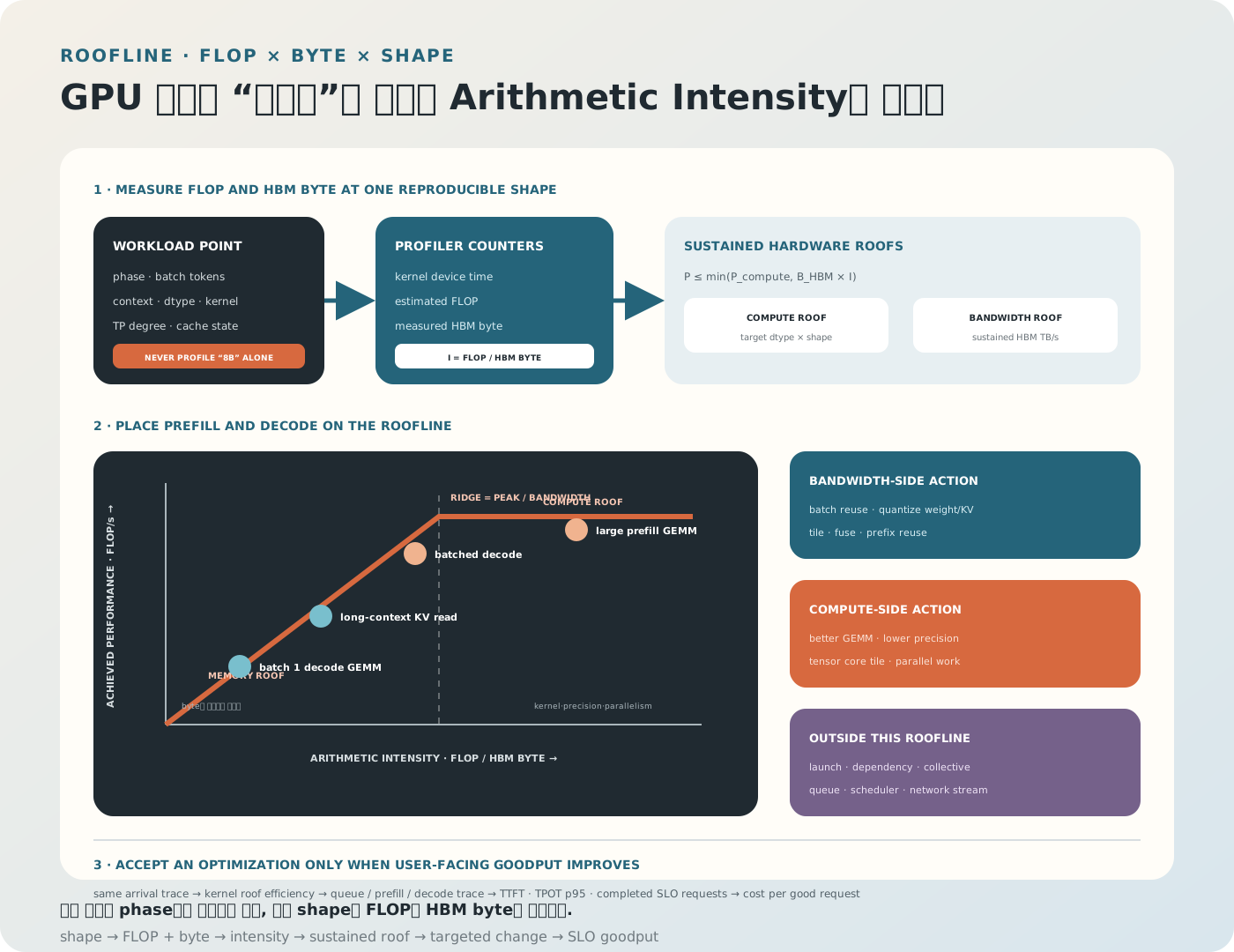
GPU Roofline 차트에서 memory bandwidth 사선과 peak compute 수평선이 ridge point에서 만나고, 작은 batch decode와 KV attention은 bandwidth 영역에, 큰 prefill GEMM은 compute 영역에 놓이며 profiler와 사용자 SLO를 연결하는 진단 흐름

그림 1. Roofline은 “GPU가 느리다”를 FLOP와 byte의 비율로 분해한다. 다만 점 하나는 특정 model·shape·batch·dtype·kernel에서 측정한 결과여야 한다.

1. 먼저 Performance의 단위를 분리한다

LLM serving 화면에는 서로 다른 단위가 동시에 등장합니다.

관측값	단위	답하는 질문
Kernel latency	ms	이 연산 한 번이 얼마나 걸렸는가?
Throughput	token/s, request/s	일정 시간에 얼마나 처리했는가?
Compute rate	FLOP/s	실제 산술 연산을 얼마나 수행했는가?
Memory bandwidth	byte/s	HBM과 processor 사이에 얼마나 옮겼는가?
Arithmetic intensity	FLOP/byte	옮긴 데이터 한 byte를 몇 번 계산에 썼는가?
TTFT	ms/request	사용자가 첫 token을 언제 받았는가?
TPOT·ITL	ms/token	이후 token이 얼마나 안정적으로 나오는가?
Goodput	SLO 충족 request/s	빠르다고 약속한 요청을 얼마나 완료했는가?

GPU utilization = 100%는 이 중 어느 것도 정확히 대신하지 않습니다. Memory copy를 기다려도 device가 바쁠 수 있고, 작은 kernel이 연속 실행돼도 tensor core 처리량은 낮을 수 있습니다.

2. FLOP는 계산량, Byte는 이동량이다

FLOP

Floating-point operation의 수입니다. Matrix multiplication C = A × B에서 shape가 다음이라면:

A: [M, K]
B: [K, N]
C: [M, N]

Multiply와 add를 각각 한 연산으로 셀 때 대략:

FLOPs ≈ 2 × M × N × K

정확한 수는 bias, activation, normalization, attention, sampling을 더해야 합니다. 또한 논문·profiler가 fused multiply-add를 1 FLOP로 세는지 2 FLOP로 세는지 확인해야 합니다.

Byte

Kernel이 HBM에서 읽고 HBM으로 쓰는 데이터량입니다.

bytes moved
  = weight reads
  + activation reads/writes
  + KV cache reads/writes
  + intermediate tensors
  + metadata and padding

Model file 크기만 넣으면 틀립니다. Cache hit, fusion, tensor layout, repeated read, temporary buffer에 따라 실제 HBM traffic이 달라집니다.

3. Arithmetic Intensity가 두 자원을 연결한다

Arithmetic intensity I는 다음과 같습니다.

$$ I = \frac{\text{FLOPs}}{\text{bytes transferred from the measured memory level}} $$

분모의 memory level을 명시해야 합니다.

HBM roofline: FLOP / HBM byte
L2 roofline:  FLOP / L2 byte
L1 roofline:  FLOP / L1 byte

같은 kernel도 HBM에서는 높은 intensity, L2에서는 낮은 intensity로 보일 수 있습니다. 이 글에서는 serving GPU의 외부 memory 병목을 보기 위해 주로 HBM byte를 사용합니다.

직관

1 FLOP/byte: 1 byte를 옮겨 산술 연산 1개만 합니다.
100 FLOP/byte: 같은 데이터 이동으로 연산을 100개 수행합니다.
Intensity가 낮으면 memory를 기다릴 가능성이 큽니다.
Intensity가 높으면 compute unit의 처리량이 먼저 막힐 수 있습니다.

4. Roofline의 기본 식

Hardware의 compute peak를 P_peak, memory bandwidth를 B_mem, workload intensity를 I라 하면 attainable performance의 단순 상한은:

$$ P_{attainable} \leq \min(P_{peak},;B_{mem}\times I) $$

Graph를 log-log 축으로 그리면:

performance
  │                 ───────── peak compute roof
  │              ╱
  │           ╱
  │        ╱  memory bandwidth roof
  │     ╱
  └──────────────────────── arithmetic intensity

Ridge Point

두 상한이 만나는 intensity입니다.

$$ I_{ridge}=\frac{P_{peak}}{B_{mem}} $$

예를 들어 설명을 위한 가상 device가:

peak compute = 800 TFLOP/s
HBM bandwidth = 3 TB/s

라면:

ridge ≈ 800 / 3
      ≈ 267 FLOP/byte

I < 267이면 단순 모델상 bandwidth roof가 낮습니다.
I > 267이면 compute roof가 낮습니다.

이 값은 예시값입니다. Dtype별 peak, sparsity 조건, boost clock, 실제 memory bandwidth가 다르므로 target GPU에서 다시 정합니다.

5. Peak가 아니라 Sustained Roof를 써야 한다

제품 사양의 peak는 필요한 조건이 모두 맞을 때의 상한입니다.

theoretical peak
  ≠ sustained GEMM peak
  ≠ this kernel's attainable peak
  ≠ end-to-end serving throughput

보다 현실적인 순서는 다음과 같습니다.

Target dtype과 shape로 충분히 큰 GEMM을 실행해 sustained compute roof를 측정합니다.
Device memory benchmark로 sustained HBM bandwidth를 측정합니다.
해당 kernel의 FLOP와 HBM byte를 profiler counter로 구합니다.
같은 clock·power·MIG·virtualization 조건에서 비교합니다.

Power cap, thermal throttling, 다른 process, ECC, partition 설정도 roof를 바꿀 수 있습니다.

6. Linear Layer의 Decode가 Memory-bound가 되기 쉬운 이유

Transformer linear projection을 다음처럼 단순화합니다.

X: [T, K]       # 이번 iteration에서 처리할 token 수
W: [K, N]       # weight
Y: [T, N]

FLOP는:

FLOPs ≈ 2 × T × K × N

Weight byte가 지배적이고 weight를 한 번 읽어 T token이 공유한다고 단순화하면:

weight bytes ≈ K × N × bytes_per_weight

intensity from weight reuse
≈ (2 × T × K × N) / (K × N × bytes_per_weight)
≈ 2T / bytes_per_weight

BF16 weight가 2 byte라면 거친 intensity는 T FLOP/byte입니다.

한 iteration의 유효 token `T`	Weight 기준 거친 intensity
1	약 1 FLOP/byte
16	약 16 FLOP/byte
128	약 128 FLOP/byte
512	약 512 FLOP/byte

실제 계산에는 activation read/write와 cache가 들어가지만 핵심은 분명합니다. 같은 weight를 한 번 읽어 더 많은 token에 쓸수록 intensity가 커집니다.

Prefill

긴 prompt의 여러 token을 함께 처리하므로 T가 큽니다. Linear layer는 matrix-matrix multiplication에 가까워 compute를 채우기 쉽습니다.

Decode

요청 하나라면 새 token 하나만 처리하므로 T=1에 가깝습니다. Continuous batching으로 active sequence 64개를 묶으면 유효 T가 커져 weight reuse가 좋아집니다.

따라서 batching은 단순히 request를 모으는 정책이 아니라 linear layer의 arithmetic intensity를 바꾸는 수단입니다.

7. “Prefill은 Compute, Decode는 Memory”는 출발점일 뿐이다

이 문장은 유용하지만 법칙으로 고정하면 안 됩니다.

Prefill도 Memory-bound가 될 수 있다

Prompt가 짧아 GEMM shape가 작습니다.
Batch token 수가 작습니다.
작은 projection이나 elementwise kernel이 많습니다.
Intermediate tensor를 HBM에 반복 materialize합니다.
Attention IO가 sequence length에서 커집니다.

Decode도 Compute-bound가 될 수 있다

Continuous batch가 매우 큽니다.
Weight가 cache에서 재사용됩니다.
저정밀 weight로 byte는 줄었지만 compute peak도 다른 경로를 탑니다.
MoE에서 선택된 expert GEMM이 충분히 큽니다.
Speculative verification으로 여러 position을 한 번에 처리합니다.

병목은 phase 이름이 아니라 실제 shape와 measured point로 판단합니다.

8. Attention의 Byte를 따로 본다

Linear layer만 계산하면 long context의 핵심을 놓칩니다.

Prefill Attention

Sequence length L, head dimension d라면 각 head의 QKᵀ와 PV에 대략 L²d 규모 연산이 들어갑니다. Naive 구현은 L×L score matrix를 HBM에 쓰고 다시 읽어 IO가 커집니다.

FlashAttention은 attention을 tile로 계산하며 SRAM에 머무는 동안 softmax와 value accumulation을 수행해 큰 intermediate matrix의 HBM read/write를 줄입니다. 중요한 점은 attention FLOP를 근본적으로 없애서가 아니라 IO complexity를 줄여 더 높은 roof에 접근한다는 것입니다.

Decode Attention

새 query 하나가 과거 모든 key·value를 읽습니다.

per layer, per request
read K/V for current context length L
write K/V for one new token
compute attention for one query position

Context가 길수록 KV read byte가 선형으로 늘어납니다. GQA·MQA는 query head보다 KV head 수를 줄여 이 byte를 낮춥니다. KV cache quantization과 block layout도 이 roof를 바꿉니다.

9. Operational Intensity와 Arithmetic Intensity를 구분한다

문헌에서는 algorithm의 이상적 데이터 이동으로 계산한 값을 arithmetic intensity라 부르기도 하고, 실제 실행에서 측정한 traffic으로 계산한 값을 operational intensity라 부르기도 합니다. 팀에서는 정의를 고정합니다.

model intensity
  = estimated FLOPs / ideal bytes

measured intensity
  = profiler FLOPs / measured HBM bytes

두 값의 간격은 다음을 드러냅니다.

Weight가 예상보다 여러 번 읽혔다.
Fusion이 깨져 intermediate가 HBM에 materialize됐다.
Layout 변환과 padding traffic이 컸다.
Cache reuse가 예상보다 좋거나 나빴다.
Profiler의 FLOP counting convention이 다르다.

10. 한 Kernel을 Roofline 위에 놓는 절차

Step 1. Shape와 Dtype을 고정한다

model: example-8b
phase: decode
batch_sequences: 32
context_tokens_p50: 4096
weight_dtype: bf16
kv_dtype: bf16
tensor_parallel: 1
kernel: attention-backend-x

model=8B만으로는 재현할 수 없습니다.

Step 2. Warm-up과 반복을 분리한다

cold:
  weight load + JIT + graph capture + allocator growth

warm:
  steady shapes + cached kernels + stable clocks

두 결과를 모두 보관하되 섞어 평균내지 않습니다.

Step 3. Latency를 측정한다

GPU event 또는 profiler의 device duration을 사용합니다. CPU wall clock에는 queue와 launch overhead가 포함될 수 있으므로 별도 기록합니다.

Step 4. FLOP와 Byte를 얻는다

가능하면 hardware counter를 사용하고, unavailable하면 shape 기반 추정과 측정 bandwidth를 함께 기록합니다.

achieved_flops_per_s = estimated_flops / kernel_seconds
achieved_bytes_per_s = measured_hbm_bytes / kernel_seconds
measured_intensity   = estimated_flops / measured_hbm_bytes

Step 5. Roof 대비 효율을 계산한다

roof_at_I = min(sustained_compute_peak,
                sustained_hbm_bandwidth × measured_intensity)

roof_efficiency = achieved_flops_per_s / roof_at_I

Roof efficiency가 낮으면 “memory-bound이니 끝”이 아닙니다. 사선 roof에도 한참 못 미치면 coalescing, occupancy, dependency, load imbalance, launch gap을 더 봐야 합니다.

11. 간단한 계산 도구

아래 코드는 단위를 명시한 작은 진단 helper입니다.

from dataclasses import dataclass


@dataclass(frozen=True)
class Roof:
    compute_tflops: float
    bandwidth_tb_s: float

    @property
    def ridge_flop_per_byte(self) -> float:
        # TFLOP/s ÷ TB/s = FLOP/byte
        return self.compute_tflops / self.bandwidth_tb_s

    def attainable_tflops(self, intensity: float) -> float:
        return min(
            self.compute_tflops,
            self.bandwidth_tb_s * intensity,
        )


def classify(intensity: float, roof: Roof) -> str:
    if intensity < roof.ridge_flop_per_byte:
        return "bandwidth-side"
    return "compute-side"


example = Roof(compute_tflops=800.0, bandwidth_tb_s=3.0)
for intensity in [1, 32, 128, 512]:
    print(
        intensity,
        classify(intensity, example),
        example.attainable_tflops(intensity),
    )

이 코드는 performance를 예측하는 simulator가 아닙니다. 병목 가설을 만드는 첫 계산입니다.

12. Roofline 밖의 네 가지 병목

12.1 Kernel Launch와 CPU Stall

작은 kernel 수백 개 사이에 빈 구간이 생기면 device compute와 HBM 어느 roof에도 닿지 않습니다.

CPU prepare → launch → tiny kernel → sync
           gap             gap

Kernel fusion, CUDA Graph 같은 launch amortization, asynchronous scheduling을 검토합니다.

12.2 Dependency와 Occupancy

Register·shared memory 사용이 커 occupancy가 낮거나, reduction dependency가 길거나, shape가 tensor core tile에 맞지 않으면 compute roof보다 훨씬 아래에 머뭅니다.

12.3 Communication

Tensor parallel에서는 collective가 critical path에 들어옵니다.

layer time
  = local compute
  + exposed all-reduce / all-gather time
  + synchronization imbalance
  − overlapped portion

이때 network bandwidth·latency roof를 별도로 그려야 합니다.

12.4 Queue와 Scheduler

Kernel이 roof에 가까워도 scheduler queue가 길면 TTFT는 나쁩니다. 반대로 batch를 작게 해 kernel 효율이 조금 낮아져도 tail latency와 goodput이 좋아질 수 있습니다.

13. 병목별 최적화 지도를 만든다

병목 가설	먼저 확인할 측정	가능한 수단	주의할 역효과
Weight bandwidth	HBM byte, batch token, GEMM shape	continuous batching, weight quantization	Queue·ITL 증가, dequant overhead
KV bandwidth	Context별 KV read, KV head, dtype	GQA/MQA, KV quantization, cache layout	품질 저하, kernel 미지원
Attention IO	HBM traffic, score materialization	FlashAttention 계열, tiling	Shape별 fallback
Compute	Tensor core utilization, tile shape	낮은 precision, better GEMM, parallelism	수치 오차, communication 증가
Launch	CPU-GPU gap, kernel duration 분포	fusion, graph capture	Dynamic shape 제약
Communication	Collective duration, overlap	TP degree 조정, topology-aware placement	Model replica capacity 감소
Scheduler	Queue age, batch churn, preemption	iteration scheduling, chunked prefill	Fairness·tail trade-off

도구 이름부터 고르지 말고 표의 왼쪽에서 오른쪽으로 이동합니다.

14. RAG Agent Workload가 Roofline을 바꾸는 방식

RAG Agent는 단순 chat보다 shape 변동이 큽니다.

검색 근거가 Prefill을 키운다

system prompt 1K
conversation 2K
retrieved evidence 6K
tool schema 1K
total prompt 10K

Retrieval top-k와 chunk 길이는 answer quality뿐 아니라 prefill FLOP·attention IO·KV allocation을 바꿉니다.

Tool Call이 Decode를 끊는다

Agent가 JSON tool call을 생성하고 외부 작업을 기다리면 KV를 보존·offload·폐기 후 재계산할지 결정해야 합니다. GPU가 tool latency 동안 memory를 점유할 수 있습니다.

Shared Prefix가 실제 Byte를 줄인다

같은 system prompt와 tool schema를 여러 request가 공유하면 prefix caching으로 prefill compute와 KV allocation을 줄일 수 있습니다. 다만 tenant·model·tokenizer·adapter identity를 cache key에 포함해야 합니다.

Output Length가 Decode Capacity를 바꾼다

짧은 분류 답변과 긴 보고서를 request/s 하나로 섞으면 capacity model이 무너집니다. Input·output token cohort를 분리합니다.

15. 작은 실험: Batch가 Ridge를 넘는 지점 찾기

Target model·GPU에서 다음 matrix를 실행합니다.

phase: decode
context: 512, 2K, 8K, 32K
batch sequences: 1, 2, 4, 8, 16, 32, 64, 128
dtype: fixed
output: 128 tokens

각 cell에 기록합니다.

{
  "phase": "decode",
  "batch_sequences": 32,
  "context_tokens": 8192,
  "kernel_ms": 12.4,
  "estimated_tflops": 97.0,
  "measured_hbm_tb_s": 2.35,
  "arithmetic_intensity": 41.3,
  "ttft_ms": 310,
  "tpot_ms": 28,
  "slo_met": true
}

그리고 다음을 찾습니다.

Batch 증가에 따라 achieved FLOP/s가 선형으로 오르는 구간
HBM bandwidth가 포화되는 구간
Ridge 근처에서 compute roof로 전환되는 구간
Throughput은 오르지만 TPOT p95가 악화되는 구간
KV memory 때문에 더 이상 admit하지 못하는 구간

선택할 operating point는 가장 오른쪽 점이 아니라 SLO를 만족하는 goodput 최대점입니다.

16. 자주 틀리는 진단

“GPU utilization이 높으니 Compute-bound다”

Utilization은 어떤 engine이 얼마나 효율적으로 일했는지 말하지 않습니다. Achieved FLOP/s와 HBM byte를 봅니다.

“이론 bandwidth로 나누면 latency가 나온다”

Cache, access pattern, concurrency, launch, dependency를 무시한 하한일 뿐입니다.

“Prefill은 항상 Compute-bound다”

짧은 prompt·작은 batch·비효율 attention에서는 그렇지 않을 수 있습니다.

“INT4면 Byte가 4분의 1이고 속도도 4배다”

Scale·zero point·packing·dequantization과 kernel 지원을 포함해야 합니다. Compute roof도 dtype에 따라 달라집니다.

“Roofline 점이 좋아졌으니 제품도 빨라졌다”

Batch를 늘려 kernel 효율이 오르면서 queue와 tail latency가 나빠질 수 있습니다. TTFT·TPOT·goodput을 함께 봅니다.

17. 최소 구현 순서

Production trace에서 prompt·output·concurrency 분포를 추출합니다.
Request timeline을 queue·prefill·decode·stream으로 분해합니다.
Target dtype의 sustained compute와 HBM roof를 측정합니다.
대표 prefill·decode shape의 FLOP와 HBM byte를 수집합니다.
Arithmetic intensity와 roof efficiency를 계산합니다.
Launch·collective·scheduler gap을 별도 trace로 분류합니다.
병목 하나를 겨냥한 변경만 적용합니다.
같은 open-loop arrival trace로 전후를 비교합니다.
TTFT·TPOT·goodput·cost가 동시에 개선됐는지 확인합니다.
Shape·dtype·engine·driver identity와 결과를 불변 artifact로 남깁니다.

실전 체크리스트

스스로 확인하기

Q1. Arithmetic intensity가 20 FLOP/byte이고 HBM bandwidth가 2 TB/s라면 memory roof는 얼마인가?

2 TB/s × 20 FLOP/byte = 40 TFLOP/s입니다. Compute peak가 더 높더라도 단순 Roofline상 40 TFLOP/s가 먼저 제한합니다.

Q2. BF16 weight의 decode batch를 1에서 32로 키우면 왜 linear layer intensity가 커지는가?

Weight를 읽는 비용을 여러 sequence의 token이 공유해 같은 weight byte당 더 많은 multiply-add를 수행하기 때문입니다.

Q3. FlashAttention은 attention의 수학적 결과를 근사해 FLOP를 줄이는 기법인가?

기본 FlashAttention은 exact attention을 tile로 재배치해 HBM IO를 줄이는 접근입니다. 구현·dtype에 따른 수치 차이는 별도 검증해야 합니다.

Q4. Roofline상 bandwidth-bound이면 memory bandwidth가 항상 최대치에 도달하는가?

아닙니다. Access pattern, occupancy, dependency, 작은 kernel, load imbalance 때문에 bandwidth roof에도 못 미칠 수 있습니다.

Q5. Kernel Roofline만으로 TTFT를 설명할 수 없는 이유는 무엇인가?

TTFT에는 gateway, tokenization, scheduler queue, prefill, sampling, network가 포함되며 Roofline은 주로 device kernel의 compute와 memory 상한을 설명하기 때문입니다.

이번 글에서는 model execution을 FLOP와 byte로 분해했습니다. 다음 글 LLM 추론 메모리 계산: Weight·Activation·KV Cache·Workspace에서는 GPU 한 장에 무엇이 얼마나 들어가는지 byte budget을 직접 계산합니다. “Checkpoint가 올라간다”와 “목표 동시성을 수용한다”를 구분합니다.

참고문헌

Williams, Waterman, Patterson, Roofline: An Insightful Visual Performance Model for Multicore Architectures, Communications of the ACM, 2009.
Dao et al., FlashAttention: Fast and Memory-Efficient Exact Attention with IO-Awareness, 2022.
Dao, FlashAttention-2: Faster Attention with Better Parallelism and Work Partitioning, 2023.
Shah et al., FlashAttention-3: Fast and Accurate Attention with Asynchrony and Low-precision, 2024.
Yu et al., Orca: A Distributed Serving System for Transformer-Based Generative Models, OSDI 2022.
Kwon et al., Efficient Memory Management for Large Language Model Serving with PagedAttention, SOSP 2023.
Zhong et al., DistServe: Disaggregating Prefill and Decoding for Goodput-optimized Large Language Model Serving, OSDI 2024.
Usami, Vishwanath, Bethel, Prefill/Decode-Aware Evaluation of LLM Inference on Emerging AI Accelerators, 2026 preprint.

검증 메모 — 문헌과 식은 2026년 7월 16일 다시 확인했습니다. Hardware peak와 engine kernel은 빠르게 변하므로 본문의 수치는 원리를 설명하는 예시값이며, 실제 판단에는 target GPU·dtype·shape에서 측정한 sustained roof와 profiler counter를 사용해야 합니다.