Field Log · Entry
분산 LLM 추론: TP·PP·EP·Context Parallel·P/D 분리 (7/10)
오늘의 결론
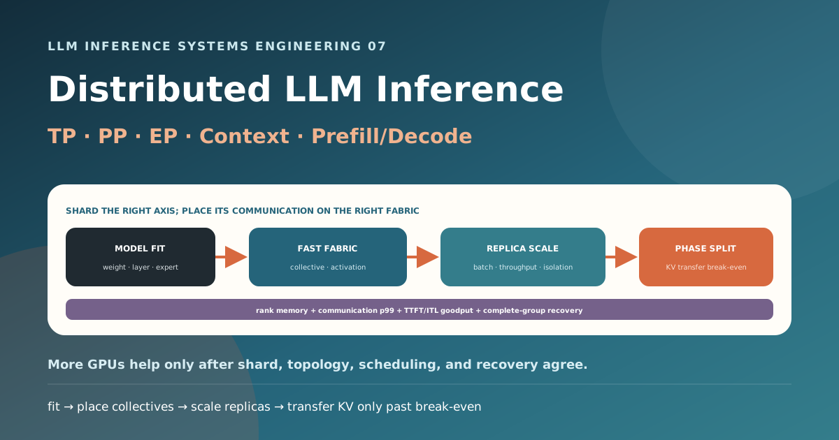
- GPU 수를 늘리는 방법은 하나가 아닙니다. Replica는 요청을, tensor parallel은 layer 안 tensor를, pipeline parallel은 layer를, expert parallel은 MoE expert를, context parallel은 sequence를 나눕니다.
- Model을 여러 GPU에 “넣는 것”과 더 빠르게 serving하는 것은 다릅니다. Shard가 memory를 줄여도 collective latency, pipeline bubble, all-to-all imbalance가 single-GPU보다 느리게 만들 수 있습니다.
- Decode는 매 token마다 작은 activation collective를 반복하므로 bandwidth뿐 아니라 network latency와 synchronization이 중요합니다. TP rank는 가능한 한 빠른 NVLink·NVSwitch failure domain 안에 둡니다.
- Prefill/decode disaggregation은 model tensor가 아니라 phase와 worker pool을 나눕니다. Interference를 줄이고 phase별 자원을 독립적으로 고를 수 있지만, 큰 KV를 옮기는 경로가 새로운 critical path가 됩니다.
- 먼저 model이 맞는 최소 parallel degree를 구하고, 그다음 SLO goodput을 위해 replica 수와 phase pool을 확장합니다. Peak token/s가 아니라 rank별 memory, collective p99, TTFT·ITL, failure recovery를 함께 release합니다.
앞 글에서는 한 target replica 안에서 serial decode step 수를 줄였습니다. 이번 글은 model weight·activation·KV와 요청을 여러 device·node에 나누는 선택을 다룹니다.
deployment objective
  → fit model + runtime + KV
  → choose the smallest model-parallel group
  → place communication on the right topology
  → add replicas for throughput
  → optionally split prefill/decode pools
  → verify SLO goodput and failure behavior
이 글에서 답하는 질문
- Replica·TP·PP·EP·context parallel은 각각 무엇을 분할하는가?
- Collective latency가 decode에 특히 민감한 이유는 무엇인가?
- Pipeline stage와 microbatch는 serving에서 어떤 bubble을 만드는가?
- MoE의 active parameter가 적어도 all-to-all이 병목인 이유는 무엇인가?
- Prefill/decode를 분리하면 어떤 KV transfer가 필요한가?
- Model 크기·topology·SLO에 맞는 parallel plan을 어떻게 검증하는가?
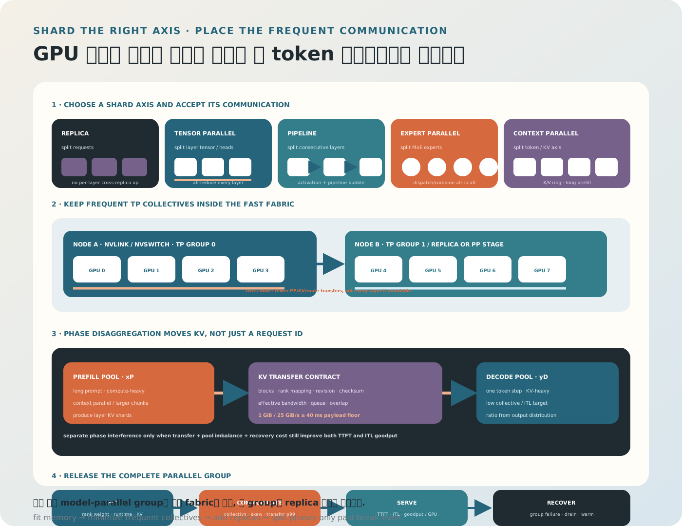
그림 1. Parallelism은 GPU 개수가 아니라 분할 축과 통신 계약이다. 가장 자주 발생하는 통신을 가장 빠른 link 안에 배치하고, model-parallel group 바깥에서 replica를 늘린다.
1. 먼저 목적을 구분한다
분산 추론을 시작하는 이유는 네 가지가 섞여 있습니다.
Memory Fit
Weight·KV·runtime이 GPU 한 장에 들어가지 않습니다.
Single-request Latency
한 요청의 prefill 또는 decode를 여러 GPU가 함께 계산해 줄이고 싶습니다.
Aggregate Throughput
동시에 더 많은 요청을 처리하고 싶습니다.
Reliability and Isolation
Tenant·model revision·SLO class를 다른 worker pool에 격리하고 싶습니다.
목적이 throughput인데 곧바로 TP를 늘리면, 독립 replica가 더 효율적인 경우가 많습니다. 반대로 model이 한 GPU에 맞지 않으면 replica 전에 model parallel이 필요합니다.
2. 분할 축 전체 지도
| 방식 | 나누는 것 | 대표 통신 | 주된 목적 |
|---|---|---|---|
| Replica / Data Parallel | Request | Router만, replica 간 없음 | Throughput·격리 |
| Tensor Parallel, TP | Layer 내부 tensor·head | All-reduce·all-gather·reduce-scatter | Weight fit·layer latency |
| Pipeline Parallel, PP | 연속 layer stage | Point-to-point activation | Weight fit·TP domain 확장 |
| Expert Parallel, EP | MoE expert | Token dispatch/combine all-to-all | Expert weight fit·sparse compute |
| Context/Sequence Parallel | Token·sequence axis | K/V ring·all-to-all | Very long prefill·context fit |
| Prefill/Decode Disaggregation | Inference phase·worker pool | KV transfer | Phase interference·resource 분리 |
현대 deployment는 이 축을 조합합니다. 예를 들어 TP=8 × PP=2 model group을 4개 replica로 띄우고, prefill group과 decode group의 개수를 다르게 둘 수 있습니다.
3. Replica가 가장 단순한 확장이다
Model 전체가 GPU 한 장에 맞는다면 independent replica를 여러 개 띄웁니다.
router
  ├─ replica 0: full model + its KV pool
  ├─ replica 1: full model + its KV pool
  └─ replica 2: full model + its KV pool
Replica 사이에는 매 layer collective가 없습니다. 요청은 한 replica에서 끝나므로 fault isolation과 scaling이 단순합니다.
대신 weight가 복제되고 prefix KV locality가 갈립니다. Router는 queue length뿐 아니라 prefix hit, adapter residency, tenant quota를 함께 봅니다.
4. Replica 수를 늘렸을 때의 함정
- 각 replica batch가 작아져 GPU 효율이 떨어질 수 있습니다.
- 동일한 hot prefix가 여러 KV pool에 중복됩니다.
- Request stickiness가 load imbalance를 만들 수 있습니다.
- Model rollout 중 revision별 replica capacity가 쪼개집니다.
- 작은 traffic에서 많은 replica는 cold graph·cache를 늘립니다.
Throughput은 replica 수에 완벽히 선형 증가하지 않습니다. Router overhead, batch dilution, shared network·CPU가 bottleneck이 됩니다.
5. Tensor Parallel은 Layer 안을 나눈다
Linear layer Y=XW의 weight를 여러 rank에 shard합니다. Megatron-LM의 전형적인 MLP 예를 단순화하면:
column-parallel first projection
W1 = [W1_0 | W1_1 | ... | W1_{P-1}]
rank r computes H_r = X W1_r

row-parallel second projection
W2 split by input rows
rank r computes partial Y_r = H_r W2_r
Y = sum_r Y_r  → all-reduce / reduce-scatter
Attention에서는 query head를 rank에 나누고 projection output을 collective로 합칠 수 있습니다. GQA의 KV head 수와 TP degree가 맞지 않으면 KV head replication 또는 uneven shard가 생길 수 있습니다.
6. TP가 줄이는 Memory
이상적인 dense weight는 rank당 대략 1/TP로 줄어듭니다.
rank weight
  ≈ sharded linear weights / TP
  + replicated norm, metadata, small tensors
  + communication buffers
KV도 attention head·layer layout에 맞춰 shard될 수 있지만 정확히 1/TP가 아닐 수 있습니다. Embedding·LM head, quantization scale, graph pool, collective workspace도 rank별로 측정합니다.
7. TP의 진짜 비용은 매 Layer Collective다
각 Transformer layer에서 partial result를 합쳐야 합니다. 80-layer model이 token마다 2번 collective를 수행한다면 한 decode token에 160번 synchronization이 생길 수 있습니다. 실제 횟수는 architecture와 fusion에 따라 다릅니다.
통신 시간을 거칠게:
α: collective launch·link·software latencyrounds: algorithm과 rank 수에 따른 단계bytes: activation payloadeffective bandwidth: topology·contention을 반영한 실효값
Decode activation이 작으면 bytes/bandwidth보다 α가 중요할 수 있습니다.
8. Collective 종류를 안다
All-reduce
모든 rank의 partial tensor를 합하고 결과를 모든 rank가 받습니다.
All-gather
각 rank의 shard를 모아 전체 tensor를 모든 rank가 갖습니다.
Reduce-scatter
합산한 결과를 shard로 나눠 각 rank에 줍니다. 다음 연산이 sharded input을 받을 수 있으면 all-reduce보다 중간 full activation을 피할 수 있습니다.
All-to-all
각 rank가 다른 모든 rank에 서로 다른 token·expert payload를 보냅니다. MoE expert parallel의 핵심입니다.
Point-to-point
한 pipeline stage가 다음 stage로 activation을 전달합니다.
Profiler에서 “communication” 하나로 합치지 말고 collective type, bytes, ranks, stream, overlap을 기록합니다.
9. TP Degree를 무작정 키우면 안 된다
TP가 커질수록 rank당 GEMM은 작아지고 collective participant는 늘어납니다.
benefit:
  weight / rank ↓ · local GEMM latency ↓

cost:
  GEMM tile efficiency ↓ · collective latency ↑
  synchronization / straggler exposure ↑
Model이 맞는 최소 TP에서 시작하고 TP=1,2,4,8의 TTFT·ITL·goodput과 rank memory를 비교합니다. 같은 총 GPU 수라면 TP=8 × replica 1과 TP=4 × replica 2가 다른 결과를 냅니다.
10. TP는 빠른 Topology 안에 둔다
일반적인 우선순위:
same GPU package / high-speed fabric
  → same node NVLink/NVSwitch
  → cross-node InfiniBand/RoCE
  → ordinary Ethernet
하드웨어 이름보다 topology matrix와 실효 collective를 측정합니다. Node 사이 TP는 매 token 통신 latency를 지불하므로, 가능하면 node 안에서 TP를 닫고 node 바깥은 PP·replica·phase transfer에 사용합니다.
11. Pipeline Parallel은 Layer를 나눈다
Layer를 연속 stage로 분할합니다.
stage 0 · GPU group A: embedding + layers 0..19
stage 1 · GPU group B: layers 20..39
stage 2 · GPU group C: layers 40..59
stage 3 · GPU group D: layers 60..79 + LM head
각 stage는 자기 layer weight와 해당 layer의 KV를 저장합니다. Stage boundary에서는 hidden activation을 다음 stage로 보냅니다.
TP처럼 매 layer 전체 rank collective를 cross-node에 수행하지 않고, stage당 boundary transfer만 하므로 큰 model을 여러 node에 걸칠 때 유리할 수 있습니다.
12. Pipeline Bubble
한 microbatch만 있으면 stage 1이 시작할 때 stage 0은 다음 일을 기다릴 수 있습니다.
time →
stage 0: [mb0] [mb1] [mb2] [mb3]
stage 1:       [mb0] [mb1] [mb2] [mb3]
stage 2:             [mb0] [mb1] [mb2] [mb3]
여러 microbatch를 흘리면 steady-state utilization은 좋아지지만 fill·drain bubble은 남습니다. Online serving에서는 request latency, continuous batch shape, stage queue가 microbatch를 제한합니다.
13. PP에서 가장 느린 Stage가 전체를 결정한다
Layer 수만 균등하게 나눠도 stage cost가 같지 않을 수 있습니다.
- Embedding과 LM head가 특정 stage에 있습니다.
- MoE layer와 dense layer 비용이 다릅니다.
- KV context length와 attention kernel이 다를 수 있습니다.
- Stage별 TP group topology가 다를 수 있습니다.
- Activation send·receive overlap이 다릅니다.
Stage latency와 memory를 profile해 layer boundary를 재배치합니다. max(stage time)가 pipeline clock을 결정합니다.
14. TP와 PP를 조합한다
16 GPU, node당 8 GPU 환경의 예:
TP = 8 within each node
PP = 2 across two nodes

stage 0: node A, 8-way TP, early layers
stage 1: node B, 8-way TP, late layers
Frequent layer collective는 node 안 NVLink에 두고, stage activation만 node 사이에 보냅니다. 단, 두 node 중 하나가 실패하면 전체 16-GPU replica가 실패합니다.
15. Expert Parallel은 MoE Expert를 나눈다
Mixture-of-Experts layer는 router가 token마다 일부 expert를 선택합니다.
hidden tokens on all ranks
  → router top-k expert IDs
  → dispatch all-to-all
  → local expert MLP
  → combine all-to-all
  → weighted output
Expert weight를 여러 rank에 나누면 resident parameter를 분산할 수 있습니다. 하지만 token payload가 expert owner로 이동하므로 all-to-all이 critical path가 됩니다.
16. MoE에서 Active Parameter만 보면 안 된다
Token 하나는 expert 2개만 활성화해도 cluster에는 많은 expert weight가 resident합니다.
compute per token → selected experts
memory footprint   → all resident expert shards
network traffic    → routed token activations
Batch가 작으면 expert별 token 수가 적어 GEMM이 작고, 인기 expert로 routing이 몰리면 일부 rank가 straggler가 됩니다. Padding을 쓰면 compute를 낭비하고, dropless block-sparse kernel은 dynamic shape를 효율적으로 다뤄야 합니다. MegaBlocks는 이러한 sparse block computation 문제를 다룹니다.
17. Expert Load Imbalance
관찰할 값:
- Expert별 routed token histogram
- Top-k overlap과 duplicate route
- Rank별 dispatch·combine byte
- Expert GEMM batch token
- Capacity overflow·token drop 여부
- Shared expert와 replicated expert 비용
- All-to-all p50·p99와 straggler rank
Training에서 균형이 좋았어도 production 언어·도메인·prompt가 달라지면 routing skew가 생길 수 있습니다. RAG의 특정 산업 용어가 일부 expert를 계속 hot하게 만들 수도 있습니다.
18. Context Parallel은 Token 축을 나눈다
아주 긴 prefill은 sequence와 KV를 device에 분할할 수 있습니다. Ring Attention은 Q block을 local하게 처리하면서 K/V block을 ring으로 전달하고 communication과 blockwise attention compute를 overlap하는 방향을 제시합니다.
rank 0 owns tokens 0..S-1
rank 1 owns tokens S..2S-1
...
K/V blocks circulate around the ring
이는 model weight를 나누는 TP와 다릅니다. 긴 prefill memory·attention을 확장할 수 있지만, 짧은 decode query가 매 token마다 distributed KV를 읽는 경로는 별도 병목이 될 수 있습니다. Prefill 전용 context parallel과 decode KV placement를 구분합니다.
19. Sequence Parallel이라는 이름의 혼동
Framework마다 sequence parallel은 다음 중 다른 의미로 쓰일 수 있습니다.
- TP 사이에서 activation의 sequence dimension을 shard
- Long-context attention을 token axis로 분산
- Ring/context parallel과 유사한 full sequence 분할
설정 이름만 보지 말고 다음 tensor contract를 문서화합니다.
tensor name · global shape · shard axis
owner ranks · collective before/after op
replicated or partitioned KV
20. Prefill/Decode Disaggregation
Prefill은 큰 token batch로 compute-bound, decode는 작은 step과 긴 KV read로 memory·latency-bound가 되기 쉽습니다. 같은 worker에 두면 긴 prefill이 decode ITL을 방해하고 phase별 parallel degree를 따로 고르기 어렵습니다.
Disaggregation은 worker pool을 나눕니다.
request → prefill pool
  → compute prompt KV + first-token state
  → transfer KV and metadata
  → decode pool
  → generate remaining tokens
DistServe와 Splitwise는 phase-specific resource·parallelism을 설계하고 interference를 제거하는 방향을 제시합니다.
21. KV Transfer를 먼저 계산한다
Disaggregation의 최소 transfer byte는 request KV 크기와 같습니다.
2편 예시의 128KiB/token model에서 8K prompt KV는 1GiB입니다. Effective 25GiB/s라면 순수 payload만 최소 약 40ms입니다.
transfer latency
  = source ready delay
  + metadata / registration
  + bytes / effective bandwidth
  + destination placement
  + queue and synchronization
TP rank별 KV shard를 decode group의 대응 rank로 보내는 topology, block layout 변환, retry도 포함합니다.
22. KV Transfer와 Compute를 Overlap한다
전체 prefill이 끝난 뒤 1GiB를 한 번에 보내면 TTFT에 transfer가 그대로 더해집니다. Layer·block 단위로 ready KV를 stream하고 network와 remaining prefill을 overlap할 수 있습니다.
하지만 너무 작은 transfer는 bandwidth를 채우지 못하고 metadata·doorbell overhead가 커집니다.
chunk too small → latency/IOPS bound
chunk too large → no overlap, TTFT spike
Mooncake는 KVCache-centric disaggregated architecture와 memory tier·scheduler·transfer를 함께 다루는 사례입니다.
23. Prefill Pool과 Decode Pool 비율
1P:1D는 기본값일 뿐입니다. 필요한 pool capacity는 workload에 따라 다릅니다.
prefill work / request ≈ input tokens and attention cost
decode work / request  ≈ output tokens × per-step context cost
RAG QA는 긴 input·짧은 output으로 prefill-heavy할 수 있고, reasoning model은 output이 길어 decode-heavy할 수 있습니다. Prompt·output joint distribution과 phase service rate로 xP:yD를 계산하고 queue를 관찰합니다.
24. Disaggregation의 새 Failure Mode
- Prefill은 끝났지만 KV transfer가 실패했습니다.
- Decode worker가 KV 일부만 받았습니다.
- Source가 block을 너무 일찍 free했습니다.
- Model·tokenizer·KV layout revision이 다릅니다.
- Decode pool이 포화돼 transferred KV가 대기하며 memory를 점유합니다.
- Retry가 같은 request KV를 중복 생성·전송합니다.
- Network partition 중 user deadline이 지났습니다.
KV object에 immutable identity, expected blocks·bytes, checksum, model revision, owner lease를 넣고 idempotent transfer·cleanup을 설계합니다.
25. Topology를 숫자로 모델링한다
Inventory 예:
node:
  gpus: 8
  intra_node:
    fabric: NVSwitch
    collective_profile: measured
  inter_node:
    fabric: 8x400G-RoCE
    oversubscription: measured
placement:
  tp_group: within_node
  pp_edge: cross_node_allowed
  expert_group: same_fabric_island
  kv_transfer: dedicated_qos_class
Vendor peak bandwidth가 아니라 message-size별 all-reduce·all-to-all·point-to-point p50·p99를 측정합니다. NIC affinity, NUMA, PCIe switch, concurrent traffic도 topology 일부입니다.
26. Communication과 Compute Overlap
비동기 stream을 쓴다고 자동으로 overlap되지는 않습니다.
- 다음 compute가 collective 결과를 바로 필요로 합니까?
- GEMM과 network가 같은 memory bandwidth를 경쟁합니까?
- GPU Direct path가 실제로 사용됩니까?
- Communication buffer가 contiguous·aligned합니까?
- NCCL/RDMA stream priority가 decode를 굶기지 않습니까?
- 다른 replica의 collective가 같은 fabric을 사용합니까?
Timeline에서 compute, collective, idle gap을 보고 exposed communication time을 계산합니다.
27. Straggler가 모든 Rank를 멈춘다
Collective는 가장 늦은 rank를 기다립니다. 한 GPU의 thermal throttling, corrected error, competing process, NUMA misplacement가 group 전체 ITL p99를 올릴 수 있습니다.
관찰할 것:
- Rank별 kernel·collective 시작/종료 timestamp
- Barrier wait skew
- GPU clock·power·ECC·Xid
- NIC retry·congestion·packet loss
- Stage queue depth
- Expert routing skew
평균 GPU utilization이 아니라 slowest-rank critical path를 봅니다.
28. Fault Domain과 Recovery
16-GPU TP×PP replica는 GPU 한 장 실패에도 전체 replica를 재시작할 수 있습니다. Replica group이 클수록 model fit은 쉬워지지만 failure blast radius와 warm-up 시간이 커집니다.
Recovery 설계:
- Health check는 rank 하나가 아니라 group consistency를 봅니다.
- Router는 degraded group에 새 request를 보내지 않습니다.
- In-flight request를 retry할 때 idempotency와 streaming 중복을 처리합니다.
- Prefix·session KV가 사라졌을 때 recompute budget을 둡니다.
- Rolling update는 old/new parallel group capacity를 동시에 감당합니다.
- Spare capacity는 GPU 수가 아니라 완전한 group 단위로 계산합니다.
29. Heterogeneous GPU를 섞을 때
서로 다른 GPU를 같은 synchronous TP group에 넣으면 느린 rank가 clock을 결정하고 kernel·dtype 지원도 달라질 수 있습니다. Heterogeneity는 보통 다음 경계가 낫습니다.
- 다른 replica pool
- Prefill과 decode phase pool
- Draft와 target pool
- Offline·best-effort class
- KV storage·transfer tier
Splitwise는 phase 특성에 맞춰 서로 다른 class의 machine을 배치하는 관점을 포함합니다. 실제 cost와 SLO를 함께 최적화합니다.
30. RAG Agent 배치에서 달라지는 것
Long Retrieved Context
Prefill pool과 context parallel 수요가 커집니다. Top-k를 늘리기 전에 quality gain 대비 prefill GPU·KV transfer cost를 계산합니다.
Short Tool Outputs
Decode가 짧아 P/D transfer 비용을 amortize하지 못할 수 있습니다. 짧은 tool-call endpoint는 colocated worker가 더 빠를 수 있습니다.
Reasoning Output
긴 decode는 decode pool과 KV bandwidth를 오래 점유합니다. Reasoning class를 별도 replica나 priority로 분리합니다.
Tool Wait and Resume
Session KV가 어느 decode worker에 있는지 routing하거나 shared KV tier에서 reload합니다. Sticky routing과 load balance를 비교합니다.
Parallel Agent Branches
공통 prefix는 공유해도 branch suffix마다 KV가 늘어납니다. Branch fan-out을 tenant quota와 group capacity에 포함하고 cancel을 모든 rank에 전달합니다.
31. 대표 Configuration 사고 실험
8B Quantized Model, 한 GPU에 Fit
start: TP=1, PP=1, multiple replicas
reason: no collective, simple failure domain
70B BF16, 한 Node 8 GPU에 Fit
start: smallest TP that fits, often 4 or 8 as measured
compare: TP=4 × 2 replicas vs TP=8 × 1 replica
140B Dense, 두 Node 필요
candidate: TP=8 within node × PP=2 across nodes
verify: stage balance, boundary activation, recovery group size
Large MoE
candidate: TP for shared dense parts + EP for experts
verify: all-to-all topology, routing skew, expert GEMM size
이는 시작점일 뿐입니다. Quantization·GQA·KV·SLO·fabric에 따라 답이 달라집니다.
32. Parallel Plan Manifest
model:
  revision: "<sha>"
  dtype: bf16
  weight_gib: "<measured>"
parallel:
  tensor: 8
  pipeline: 2
  expert: 1
  context: 1
  replicas: 4
phase:
  colocated: true
placement:
  tp_within_node: true
  pp_edges: [[node_a, node_b]]
runtime:
  kv_layout: "<version>"
  max_batched_tokens: "<value>"
  max_active_sequences: "<value>"
network:
  collective_profile_id: "<artifact>"
release:
  engine_commit: "<sha>"
  driver_firmware: "<versions>"
Plan과 실제 rank mapping을 함께 artifact로 보존합니다.
33. 무엇을 Benchmark할까
Primitive
- Message-size별 all-reduce·all-gather·reduce-scatter
- Expert all-to-all under skew
- Point-to-point activation
- KV block transfer·layout conversion
Model Iteration
- Prefill·decode phase별 rank time
- TP degree별 kernel과 exposed collective
- PP stage clock과 bubble
- EP expert batch와 straggler
- Context length별 attention communication
Serving
- TTFT·ITL·end-to-end p50·p95·p99
- Input·output token goodput/GPU
- Queue depth by replica·stage·phase
- KV transfer latency·failure
- Prefix locality와 batch size
- Power·cost per SLO-attaining request
Recovery
- Rank failure detection
- Group drain·restart·warm-up
- Retry success와 duplicate stream
- Rolling update capacity
34. 선택 절차
- Rank별 weight·runtime·KV memory를 계산합니다.
- Model이 맞는 최소 TP·PP·EP combination을 찾습니다.
- Topology microbenchmark로 frequent collective placement를 정합니다.
- Target prefill·decode shape에서 parallel degree를 sweep합니다.
- 같은 GPU 수로 model-parallel과 replica trade-off를 비교합니다.
- Stage·expert·rank imbalance를 profile합니다.
- Production prompt·output 분포로 phase work ratio를 계산합니다.
- Colocation의 TTFT·ITL interference를 측정합니다.
- 필요한 경우 P/D 분리와 KV transfer break-even을 시험합니다.
- Prefix routing·tenant fairness·Agent session locality를 추가합니다.
- Open-loop load에서 SLO goodput과 fabric contention을 봅니다.
- Failure·rolling update를 완전한 parallel group 단위로 검증합니다.
실전 체크리스트
- 분산 목적이 memory fit·latency·throughput·isolation 중 무엇인지 적었다.
- Model이 맞는 최소 model-parallel degree부터 시작한다.
- Replica와 tensor parallel의 throughput 차이를 비교했다.
- TP의 layer당 collective type·횟수·bytes를 안다.
- GQA KV head와 TP shard·replication을 확인했다.
- TP group을 가능한 한 빠른 fabric 안에 배치했다.
- PP stage별 layer·memory·latency를 균형화했다.
- Pipeline fill·drain bubble과 microbatch를 측정했다.
- MoE expert별 token과 all-to-all skew를 기록한다.
- Token drop·padding·dropless kernel policy가 명시돼 있다.
- Context parallel의 prefill 이득과 decode 비용을 분리했다.
- Framework의 sequence parallel 의미를 tensor contract로 적었다.
- P/D 분리 전 KV byte와 transfer lower bound를 계산했다.
- KV chunk 크기와 compute/transfer overlap을 측정했다.
- Prefill·decode pool 비율을 실제 input/output 분포로 정했다.
- Vendor peak가 아니라 collective·transfer p99를 측정했다.
- Slowest rank와 exposed communication time을 관찰한다.
- Failure spare를 완전한 parallel group 단위로 보유한다.
- RAG Agent의 short tool·long reasoning class를 분리해 본다.
- SLO goodput/GPU와 cost로 최종 plan을 선택한다.
스스로 확인하기
Q1. Model이 한 GPU에 들어가는데 throughput을 늘리려면 TP가 첫 선택인가?
대개 independent replica가 더 단순한 시작점입니다. TP는 매 layer collective를 추가합니다. 다만 single-request latency, very large batch kernel, memory headroom 같은 이유로 TP가 유리한지는 측정해야 합니다.
Q2. Tensor parallel과 pipeline parallel의 통신 차이는 무엇인가?
TP는 layer 내부 partial tensor를 합치기 위해 자주 collective합니다. PP는 연속 layer stage 사이에서 activation을 point-to-point로 전달하지만 pipeline bubble과 stage imbalance가 생깁니다.
Q3. MoE가 active parameter가 적으면 network도 적게 쓰는가?
반드시 그렇지 않습니다. Token activation을 선택된 expert owner로 dispatch하고 다시 combine하는 all-to-all이 필요하며 routing skew가 특정 rank를 병목으로 만들 수 있습니다.
Q4. Prefill/decode를 분리하면 interference가 완전히 공짜로 사라지는가?
아닙니다. 두 phase compute interference는 줄지만 prompt 전체 KV transfer, pool imbalance, layout compatibility, failure·retry가 새 비용이 됩니다.
Q5. Network bandwidth가 높으면 decode TP가 항상 잘 scale하는가?
아닙니다. 작은 activation collective를 layer마다 반복하면 bandwidth보다 per-collective latency와 synchronization, slowest-rank skew가 지배할 수 있습니다.
다음 글
이번 글은 model과 request를 여러 device에 배치했습니다. 다음 글 저정밀 LLM 추론: FP8·INT8·INT4·FP4 Kernel과 Calibration에서는 각 rank의 weight·activation·KV byte와 tensor core 경로를 줄이면서 정확도를 지키는 방법을 다룹니다.
참고문헌
- Shoeybi et al., Megatron-LM: Training Multi-Billion Parameter Language Models Using Model Parallelism, 2019.
- Aminabadi et al., DeepSpeed Inference: Enabling Efficient Inference of Transformer Models at Unprecedented Scale, SC 2022.
- Zhong et al., DistServe: Disaggregating Prefill and Decoding for Goodput-optimized Large Language Model Serving, OSDI 2024.
- Patel et al., Splitwise: Efficient Generative LLM Inference Using Phase Splitting, ISCA 2024.
- Qin et al., Mooncake: Trading More Storage for Less Computation — A KVCache-centric Architecture for Serving LLM Chatbot, FAST 2025.
- Gale et al., MegaBlocks: Efficient Sparse Training with Mixture-of-Experts, MLSys 2023.
- Liu et al., Ring Attention with Blockwise Transformers for Near-Infinite Context, 2023.
- Kwon et al., Efficient Memory Management for Large Language Model Serving with PagedAttention, SOSP 2023.
검증 메모 — 개념과 문헌은 2026년 7월 16일 확인했습니다. Parallel primitive의 실제 collective·KV shard·graph 지원은 model architecture와 engine revision에 따라 다릅니다. 본문의 rank·layer·bandwidth 수치는 원리를 설명하는 예시값이며 target topology에서 message-size별 communication, rank memory, TTFT·ITL·goodput과 recovery를 다시 측정해야 합니다.
Reader questions
읽으며 남긴 질문
글을 읽으며 붙잡아 둔 질문입니다. 다시 살펴보거나, 보내지 않은 질문을 한 번에 블로그 주인에게 전달할 수 있습니다.