Field Log · Entry
Transformer 추론 커널: GEMM·Attention·FlashAttention·Fusion (3/10)
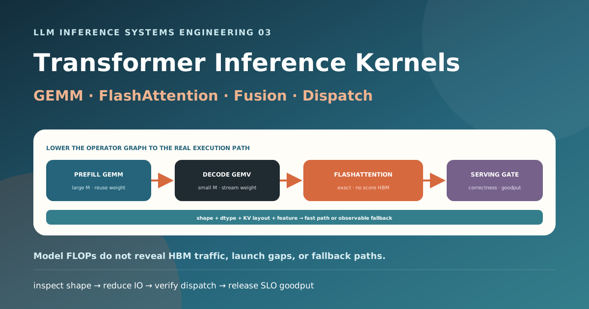
오늘의 결론
- Transformer 수식은 GPU에서 그대로 실행되지 않습니다. Framework가 operator graph를 만들고, serving engine이 shape·dtype·mask·KV layout에 맞는 kernel을 선택해 launch합니다.
- Prefill의 projection은 token 행이 큰 GEMM이지만 decode는 매 step의 token 행이 작아 GEMV에 가까워집니다. 같은 weight를 사용해도 arithmetic intensity와 batch 효과가 다릅니다.
- FlashAttention은 attention을 근사하지 않습니다. Tile별 online softmax로 중간 score matrix의 HBM materialization을 피하는 exact IO-aware algorithm입니다.
- Fusion은 launch와 HBM 왕복을 줄이지만 모든 조합을 지원하지는 않습니다. Head dimension, dtype, GQA, page table, mask가 달라지면 다른 kernel이나 느린 fallback으로 갈 수 있습니다.
- 빠른 microbenchmark는 필요조건일 뿐입니다. 수치 정확성, cold JIT, scheduler, KV paging, CUDA Graph, 실제 prompt·output 분포를 포함한 end-to-end goodput으로 release해야 합니다.
앞 글에서는 GPU HBM을 weight·runtime·KV cache·headroom으로 나눠 계산했습니다. 이번 글은 그 byte가 한 Transformer step에서 어떻게 읽히고 쓰이는지 kernel 수준으로 내려갑니다.
model architecture
  → operator graph
  → shape + dtype + layout
  → kernel dispatch / fusion / graph replay
  → device execution
  → latency · throughput · numerical result
이 글에서 답하는 질문
- Transformer block 하나는 어떤 GPU kernel들로 실행되는가?
- Prefill과 decode에서 같은 linear layer의 성능이 왜 달라지는가?
- FlashAttention은 무엇을 계산하지 않는 것이 아니라 무엇을 저장하지 않는가?
- Fusion과 CUDA Graph는 각각 어떤 overhead를 줄이는가?
- Optimized kernel이 지원되지 않을 때 fallback을 어떻게 발견하는가?
- Microbenchmark 결과를 production serving 성능으로 어떻게 검증하는가?
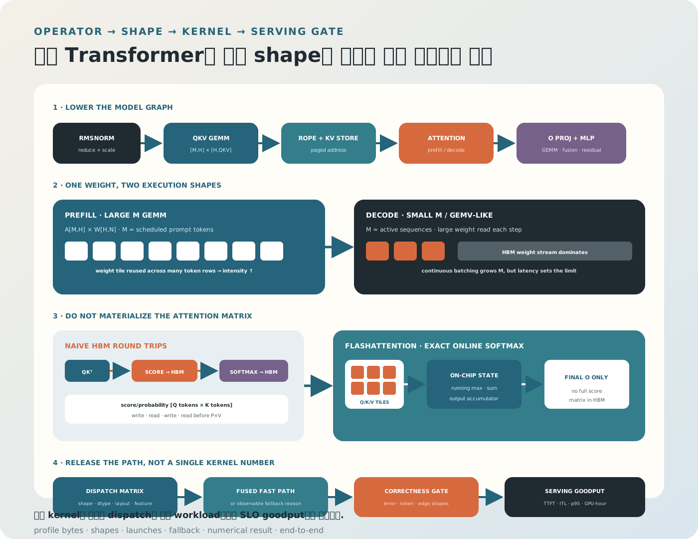
그림 1. Kernel 최적화의 단위는 모델 이름이 아니라 실제 shape·dtype·layout·기능 조합이다. 빠른 경로가 선택됐는지와 결과가 같은지를 함께 검증한다.
1. Model Graph와 Kernel Graph는 다르다
Decoder-only Transformer 한 layer를 수식으로 보면 비교적 단순합니다.
x
  → RMSNorm
  → Q/K/V projection
  → RoPE
  → causal attention
  → output projection + residual
  → RMSNorm
  → gated MLP
  → residual
하지만 GPU trace는 더 많은 launch를 보여줄 수 있습니다.
- Matrix multiplication
- Bias·scale·activation
- RMSNorm reduction
- RoPE elementwise transform
- KV cache write·gather
- Attention tile·reduction
- Residual add
- Quantize·dequantize
- Tensor-parallel collective
- Logits processing과 sampling
반대로 compiler나 library가 여러 operator를 한 kernel로 합치면 graph의 노드 수는 줄어듭니다. 따라서 “Transformer layer가 빠른가”보다 어떤 operator가 어떤 kernel로 lowering됐는가를 묻는 편이 정확합니다.
2. 한 Step의 실행 경로
설명을 위해 pre-norm, gated MLP decoder layer를 보겠습니다.
input hidden [M, H]
  ├─ RMSNorm
  ├─ QKV projection [M,H] × [H,Q+K+V]
  ├─ RoPE + KV cache store
  ├─ attention(Q, paged K/V)
  ├─ output projection [M,H] × [H,H]
  ├─ residual + RMSNorm
  ├─ gate/up projection [M,H] × [H,2I]
  ├─ SiLU × gate
  ├─ down projection [M,I] × [I,H]
  └─ residual
여기서 M은 한 iteration에 처리하는 token 행의 수입니다. Prefill에서는 여러 sequence의 prompt token 또는 chunk token 합이고, decode에서는 보통 active sequence마다 새 token 한 개입니다.
3. GEMM Shape부터 읽는다
Linear projection은 보통 다음 곱으로 표현됩니다.
M: 이번 iteration의 batch token 수K: input hidden dimensionN: output projection dimension
이때 대략적인 multiply-add 연산량은 2MKN FLOP입니다. 그러나 FLOP만으로 시간은 정해지지 않습니다. Weight·activation을 HBM에서 읽는 byte, tile reuse, tensor core 사용 여부, launch overhead가 함께 작동합니다.
4. Prefill은 큰 GEMM에 가깝다
예를 들어 16개 요청이 각각 512 prompt token을 한 번에 처리하면 M=8192입니다. 같은 weight tile이 많은 token 행에서 재사용되므로 arithmetic intensity가 커지고 tensor core를 채우기 쉽습니다.
prefill projection
M = total scheduled prompt tokens
K = hidden size
N = projection size

large M → weight reuse ↑ → compute utilization ↑
단, 32K prompt를 한 번에 넣는다고 항상 좋은 것은 아닙니다. Attention workspace와 activation peak, 다른 decode 요청의 대기 시간이 커집니다. 그래서 scheduler는 긴 prompt를 chunk로 나눌 수 있습니다.
5. Decode는 작은 M의 GEMV형 문제가 된다
Autoregressive decode는 sequence마다 한 step에 새 token 하나를 계산합니다.
decode projection
M ≈ active sequences in this iteration
K = hidden size
N = projection size
Batch가 작으면 각 layer에서 큰 weight를 읽고 적은 token만 계산합니다. Matrix-vector multiplication에 가까워지고 memory bandwidth가 병목이 되기 쉽습니다. Continuous batching이 active sequence를 모으는 이유 중 하나가 M을 키워 weight read를 공유하기 위해서입니다.
6. Batch Size보다 Batch Tokens가 정확하다
Prefill 요청 2개와 decode 요청 30개가 같은 iteration에 있으면 단순 request count는 kernel shape를 설명하지 못합니다.
scheduled requests = 32
prefill tokens      = 2 × 256
decode tokens       = 30 × 1
batch tokens M      = 542
Profile에는 최소한 prefill_tokens, decode_tokens, active_sequences, max_context, M/K/N을 함께 남깁니다. 다음 글의 scheduler도 이 token 단위 예산을 사용합니다.
7. Tensor Core Fast Path의 조건
GPU peak FLOPS는 모든 matrix shape에서 자동으로 나오지 않습니다.
- FP16·BF16·FP8·INT8 등 지원 dtype인가?
M/K/N과 leading dimension이 kernel tile에 맞는가?- Pointer alignment와 memory layout이 맞는가?
- Quantization group과 scale layout이 kernel이 기대한 형태인가?
- Transpose·padding·packing 비용이 별도로 생기지 않는가?
- GPU architecture에 맞게 compile됐는가?
예를 들어 M이 작거나 K/N이 애매하게 정렬되면 tile의 빈 lane이 늘어납니다. 이때 이론 peak 대비 achieved FLOPS가 낮아도 kernel이 나쁘다고 단정할 수 없습니다. 먼저 shape가 가진 구조적 한계를 봅니다.
8. Materialization이 HBM Traffic을 만든다
Operator를 하나씩 실행하면 중간 tensor를 HBM에 썼다가 다음 kernel이 다시 읽을 수 있습니다.
RMSNorm output  → HBM write → QKV GEMM read
bias output     → HBM write → activation read
residual output → HBM write → next norm read
중간 tensor가 X byte라면 불필요한 materialization 한 번은 대략 X byte write와 X byte read를 더합니다. Kernel launch overhead도 추가됩니다. Memory-bound decode에서는 작은 FLOP 절감보다 이 왕복 제거가 더 중요할 수 있습니다.
9. Fusion의 세 종류
Epilogue Fusion
GEMM accumulator에 bias·activation·scale을 적용한 뒤 최종 결과만 저장합니다.
GEMM → bias → SiLU → storeElementwise Fusion
Residual add와 RMSNorm처럼 같은 tensor를 연속해 읽는 연산을 합칩니다.
residual add + RMSNorm + quantizeStructural Fusion
Q·K·V projection을 하나의 큰 matrix multiplication으로 묶거나 gate·up projection을 함께 계산합니다.
three launches: xWq, xWk, xWv
one launch:     x[Wq | Wk | Wv]
Fusion은 launch 수와 HBM traffic을 줄이지만 register pressure, occupancy, compile variant 수를 키울 수 있습니다. “가능한 모든 것을 합친다”가 아니라 target shape에서 측정합니다.
10. Attention의 단순 구현
Scaled dot-product attention은 다음과 같습니다.
단순 구현은 큰 score matrix를 materialize할 수 있습니다.
QKᵀ        → score [query_tokens, key_tokens]를 HBM에 저장
mask/scale → score를 다시 읽고 저장
softmax    → probability를 다시 읽고 저장
P × V      → probability를 읽고 output 계산
Sequence가 길어지면 score와 probability의 HBM 이동이 attention 시간을 지배합니다. 문제는 수식의 FLOP만이 아니라 intermediate tensor의 읽기·쓰기입니다.
11. FlashAttention은 Exact Attention이다
FlashAttention은 Q·K·V를 SRAM에 맞는 tile로 나누고, score block을 만든 뒤 바로 online softmax 통계와 output accumulator에 반영합니다. 전체 score matrix를 HBM에 저장하지 않습니다.
for each Q tile:
  keep output accumulator + running max + running sum on chip
  for each K/V tile:
    load K/V tile
    compute score tile
    update online softmax statistics
    update output accumulator
  write final output once
핵심은 attention을 계산하지 않는 것이 아니라 같은 exact result를 다른 I/O schedule로 계산하는 것입니다. 원 논문은 이를 IO-aware exact attention으로 설명하고 HBM과 on-chip SRAM 사이의 이동을 분석합니다.
12. Online Softmax의 핵심
각 tile의 local maximum과 exponential sum을 구하고, 더 큰 maximum이 나타나면 이전 accumulator를 rescale합니다.
기존 block까지의 통계를 (m, l)이라 하고 새 block의 maximum과 합을 (m_b, l_b)라 하면:
Output accumulator도 같은 scale로 보정합니다. 이렇게 하면 모든 score를 보관하지 않고도 전체 row의 안정적인 softmax를 얻습니다.
13. Prefill Attention과 Decode Attention은 다르다
Prefill
Query token과 key token이 모두 많습니다. Causal mask 아래의 큰 attention matrix를 tile하고 Q·K·V reuse와 tensor core 활용이 중요합니다.
Decode
Sequence마다 query는 보통 한 token이지만 과거 K/V context는 깁니다.
query length = 1
key length   = current context length
Decode attention은 paged KV block을 gather하며 긴 context를 scan합니다. Query head가 여러 KV head를 공유하는 GQA, 서로 다른 sequence length, page table indirection 때문에 prefill과 다른 kernel·load balancing이 필요합니다.
14. Paged KV는 Kernel Interface도 바꾼다
KV가 연속 tensor라면 address 계산이 단순합니다. Paged KV에서는 logical token position을 physical block과 offset으로 변환해야 합니다.
logical position
  → block_table[sequence, logical_block]
  → physical_block_id
  → K/V base + offset
이 indirection은 메모리 낭비를 줄이는 대신 kernel이 page table과 불연속 block을 다뤄야 함을 뜻합니다. Page size가 너무 작으면 metadata와 address overhead가 늘고, 너무 크면 마지막 block의 내부 fragmentation이 커집니다.
15. GQA는 Head Mapping을 요구한다
Grouped-Query Attention에서는 여러 query head가 하나의 KV head를 공유합니다.
query heads: 32
KV heads:     8
group size:   4 query heads / KV head
Kernel은 동일한 K/V tile을 query head group 사이에서 재사용할 수 있습니다. 하지만 TP shard, head dimension, group size 조합이 fast path 제약과 맞지 않으면 KV replication 또는 별도 fallback이 생길 수 있습니다.
16. Split-KV와 Load Balancing
Decode context length가 매우 길거나 sequence별 길이 편차가 크면 한 CTA가 긴 sequence를 독점할 수 있습니다. KV dimension을 여러 작업으로 나눠 부분 output·softmax 통계를 계산하고 마지막에 reduce하는 방식을 사용할 수 있습니다.
long KV range
  → split 0 partial (m₀, l₀, O₀)
  → split 1 partial (m₁, l₁, O₁)
  → ...
  → numerically stable merge
Split을 늘리면 parallelism은 커지지만 partial buffer와 reduction 비용도 늘어납니다. FlashInfer는 다양한 KV layout과 workload를 위한 composable attention 및 load-balanced scheduling을 다룹니다.
17. FlashAttention 세대의 방향
FlashAttention
Tiling과 recomputation으로 exact attention의 HBM I/O를 줄였습니다.
FlashAttention-2
Non-matmul FLOP를 줄이고 thread block·warp 사이의 work partition을 개선해 GPU 활용도를 높였습니다.
FlashAttention-3
Hopper의 asynchronous execution, warp specialization, Tensor Memory Accelerator를 활용하고 FP8 attention 경로를 확장했습니다.
이름의 숫자만 올린다고 현재 engine이 새 kernel을 쓰는 것은 아닙니다. GPU architecture, package build, head dimension, mask 기능과 dispatch log를 확인해야 합니다.
18. FlashInfer가 Serving에 더하는 것
Serving attention은 연구용 고정 shape와 다릅니다.
- Sequence마다 context length가 다릅니다.
- KV가 paged 또는 ragged layout입니다.
- Prefill과 decode가 섞입니다.
- Custom mask, RoPE, logits transform이 필요할 수 있습니다.
- CUDA Graph와 dynamic request scheduling을 함께 써야 합니다.
FlashInfer는 block-sparse 형식을 포함한 composable KV representation, customizable JIT template, load-balanced scheduling을 serving attention engine 관점에서 제시합니다. 중요한 교훈은 “최고의 attention kernel 하나”가 아니라 workload별 dispatch 체계입니다.
19. Dispatch Matrix를 명시한다
Fast path는 다음 축의 조합으로 결정될 수 있습니다.
| 축 | 예시 |
|---|---|
| Phase | prefill, chunked prefill, decode |
| Dtype | FP16, BF16, FP8, INT8 KV |
| Head | head dimension, Q heads, KV heads |
| KV layout | contiguous, paged, ragged, quantized |
| Mask | causal, sliding window, custom sparse |
| Position | RoPE variant, scaling, offset |
| Hardware | Ampere, Ada, Hopper, Blackwell |
| Feature | prefix share, speculative tree, grammar |
Release artifact에 “지원한다”라는 문장만 두지 말고 (engine revision, GPU, shape, feature) → kernel name 표를 남깁니다.
20. Fallback은 정확하지만 느릴 수 있다
Optimized kernel이 지원하지 않는 조합에서는 framework reference path, 여러 개의 unfused kernel, 다른 attention backend로 돌아갈 수 있습니다.
requested feature
  → fast path predicate false
  → generic fallback
  → result is correct
  → latency silently regresses
이 문제는 crash가 없어 놓치기 쉽습니다. Profiler와 engine log에서 kernel name, launch count, graph capture 여부, fallback reason을 metric으로 만듭니다.
21. CUDA Graph가 줄이는 것은 Launch Overhead다
CPU가 매 decode step마다 수백 개 kernel을 개별 launch하면 GPU가 계산을 끝내고 다음 command를 기다릴 수 있습니다. CUDA Graph는 반복되는 launch sequence를 capture해 한 번에 replay합니다.
그러나 captured graph는 shape와 memory address에 제약이 있습니다.
dynamic active batch
  → pad to captured bucket
  → replay graph
  → mask inactive slot
Bucket이 너무 촘촘하면 graph memory pool과 warm-up 시간이 늘고, 너무 거칠면 padding으로 불필요한 계산이 생깁니다. CUDA Graph는 HBM traffic을 자동으로 줄이지 않으며 fusion과 역할이 다릅니다.
22. JIT와 AOT의 Trade-off
Precompiled Library
- 기동이 예측 가능합니다.
- 지원 variant가 제한될 수 있습니다.
- 검증된 kernel을 재사용하기 쉽습니다.
JIT Specialization
- Custom dtype·head dimension·feature에 맞춘 code를 만들 수 있습니다.
- 첫 요청 compile latency와 cache 관리가 필요합니다.
- Compiler·driver revision에 따라 artifact가 달라질 수 있습니다.
Production에서는 target matrix를 deploy 전에 compile·warm-up하고 cache key에 GPU architecture, compiler, template, model shape, feature flag를 포함합니다.
23. Kernel 선택 전 수치 계약을 세운다
빠른 kernel이 reference와 bitwise identical할 필요는 없지만, 허용 기준은 먼저 정해야 합니다.
- FP32 reference 대비 max·mean absolute error
- Relative error와 cosine similarity
- Attention row의 NaN·Inf 여부
- Logits top-k 순위와 margin
- Greedy generation token parity
- Sampling distribution의 통계적 차이
- 긴 context에서 error growth
FP8·quantized KV처럼 precision을 바꾸면 성능 최적화와 model quality 평가를 분리하지 않습니다.
24. Edge Case Test Matrix
Fast path만 happy path에서 시험하면 부족합니다.
sequence length: 1, page-1, page, page+1, max-context
batch:           1, bucket boundary, max active
head dim:        supported variants
mask:            causal, sliding, custom
position:        offset 0, long offset, scaled RoPE
KV:              empty, partial page, shared prefix, quantized
request:         cancel, preempt, resume, speculative branch
Page boundary와 graph bucket boundary에서 out-of-bounds, stale KV, mask 오류가 잘 드러납니다.
25. Microbenchmark Manifest
Kernel latency 숫자에는 실행 조건을 붙입니다.
hardware:
  gpu: H100-SXM-80GB
  driver: "<exact-version>"
software:
  engine_commit: "<sha>"
  cuda: "<version>"
  kernel_backend: "<name-and-version>"
shape:
  phase: decode
  batch_sequences: 64
  batch_tokens: 64
  context_tokens: [512, 4096, 16384]
  q_heads: 32
  kv_heads: 8
  head_dim: 128
  dtype: bf16
  kv_dtype: bf16
  page_size: 16
measurement:
  warmup: 200
  iterations: 2000
  clock_policy: fixed
best of 100 하나만 보고하지 말고 median, p95, 분산, cold compile을 구분합니다.
26. Device Time을 정확히 잰다
GPU launch는 asynchronous입니다. CPU wall clock으로 kernel call 전후를 바로 재면 실제 device 실행이 포함되지 않을 수 있습니다.
import torch

start = torch.cuda.Event(enable_timing=True)
end = torch.cuda.Event(enable_timing=True)

for _ in range(200):
    kernel(*inputs)  # warm-up and JIT/cache population

start.record()
for _ in range(2000):
    kernel(*inputs)
end.record()
torch.cuda.synchronize()

mean_ms = start.elapsed_time(end) / 2000
End-to-end 측정에서는 synchronization을 request path에 억지로 넣지 말고 server timestamp와 GPU profiler를 함께 사용합니다.
27. 무엇을 Profile할까
Kernel 수준
- Kernel name과 launch count
- Duration distribution
- Achieved FLOPS와 memory throughput
- Tensor core utilization
- Occupancy와 register·shared memory 사용
- HBM read·write byte
- L2 hit rate
- Warp stall reason
Iteration 수준
- Scheduled prefill·decode token
M/K/N, context length distribution- Graph replay·eager execution 비율
- Fast path·fallback count
- Collective overlap
- Idle gap과 CPU launch gap
Kernel 하나가 20% 빨라졌어도 그 kernel이 iteration의 5%라면 전체 이득은 작습니다. Amdahl의 법칙으로 end-to-end upper bound를 먼저 계산합니다.
28. Microbenchmark가 Serving을 속이는 경우
다음 실험은 실제 serving을 과대평가할 수 있습니다.
- 고정된 이상적 shape만 반복합니다.
- 모든 JIT와 graph가 이미 warm입니다.
- KV가 연속이고 cache hit가 좋습니다.
- Sequence length가 모두 같습니다.
- Scheduler·tokenization·sampling·network를 제외합니다.
- 다른 tenant의 adapter·grammar·mask variant가 없습니다.
- TP collective와 prefill interference가 없습니다.
따라서 kernel benchmark 뒤에 model iteration, offline throughput, open-loop serving load 순서로 검증 범위를 넓힙니다.
29. End-to-End Release Gate
1. reference correctness
2. exhaustive edge shapes
3. kernel microbenchmark
4. model iteration benchmark
5. scheduler + paged KV integration
6. open-loop production-shaped load
7. quality + SLO + goodput gate
최종 지표는 peak token/s만이 아닙니다.
- Time to First Token
- Inter-Token Latency
- End-to-end latency p50·p95·p99
- SLO를 만족한 input·output token/s
- Request goodput
- GPU-hour당 완료 요청
- Error·fallback·OOM·preemption rate
30. RAG Agent에서 Kernel Shape가 달라지는 지점
긴 Retrieved Context
검색 결과를 많이 붙이면 prefill GEMM과 attention이 커집니다. Chunk를 무작정 줄이는 것이 아니라 relevance gain 대비 TTFT와 KV cost를 봅니다.
공유 Tool Schema
긴 system prompt와 tool schema는 prefix cache hit 시 prefill을 줄일 수 있습니다. 하지만 model·tokenizer·schema revision이 바뀌면 새 shape와 cold path가 발생합니다.
짧은 Decode와 Tool Call
Agent는 긴 답변보다 짧은 JSON tool call을 여러 번 생성할 수 있습니다. 이 경우 decode kernel peak보다 request 전환, sampling·grammar, tool wait 뒤 resume overhead가 더 중요할 수 있습니다.
Structured Generation
Grammar mask가 매 step logits 전체에 적용되면 attention이 빨라도 sampling path가 병목이 됩니다. Vocabulary size, allowed-token representation, CPU↔GPU synchronization을 profile합니다.
Branching
Parallel plan 또는 speculative branch는 shared prefix 뒤에 여러 decode sequence를 만듭니다. Batch M은 커지지만 KV block과 scheduler cost도 늘어납니다.
31. 최적화 실험의 최소 순서
- Production trace에서 phase·batch token·context shape histogram을 만듭니다.
- Model operator graph와 current kernel trace를 연결합니다.
- Top latency·HBM traffic·launch gap을 찾습니다.
- Target shape에서 fast path predicate와 fallback reason을 확인합니다.
- Reference implementation과 수치 계약을 고정합니다.
- Fusion·attention backend·graph bucket을 하나씩 변경합니다.
- Kernel과 iteration level을 모두 측정합니다.
- Edge shape와 feature 조합 regression test를 실행합니다.
- Open-loop load에서 TTFT·ITL·goodput을 확인합니다.
- Engine·driver·kernel revision과 dispatch matrix를 함께 release합니다.
실전 체크리스트
- Model operator와 실제 kernel launch를 연결했다.
- Request 수가 아니라 prefill·decode batch token을 기록한다.
- Prefill과 decode의
M/K/N분포를 분리했다. - Dtype·alignment·tile eligibility를 확인했다.
- Intermediate HBM materialization을 찾았다.
- Fusion 전후 register·occupancy·latency를 함께 측정했다.
- FlashAttention이 exact IO-aware algorithm임을 구분했다.
- Prefill과 paged decode attention backend를 분리했다.
- GQA head mapping과 TP shard를 확인했다.
- Long-context split-KV reduction을 검증했다.
- Feature·shape별 dispatch matrix를 보관한다.
- Generic fallback count와 reason을 metric으로 만든다.
- CUDA Graph bucket의 padding과 memory 비용을 측정했다.
- JIT cold start와 compiled artifact cache를 시험했다.
- Reference 대비 수치·token·quality gate가 있다.
- Page·bucket·context boundary regression test가 있다.
- GPU event와 profiler로 asynchronous 실행을 올바르게 측정했다.
- Kernel 이득을 iteration과 end-to-end goodput에서 재검증했다.
- 실제 RAG prompt·tool·grammar 분포로 부하를 만들었다.
- Revision별 결과와 rollback 조건을 남겼다.
스스로 확인하기
Q1. Decode projection이 prefill보다 memory-bound가 되기 쉬운 이유는 무엇인가?
한 step의 token 행 M이 작아 큰 weight를 읽고도 수행하는 계산이 적기 때문입니다. Continuous batching으로 여러 active sequence를 묶으면 weight reuse와 arithmetic intensity를 높일 수 있습니다.
Q2. FlashAttention은 attention score를 근사하거나 생략하는가?
아닙니다. Tile별 online softmax로 exact attention을 계산하되 전체 score·probability matrix를 HBM에 materialize하지 않아 I/O를 줄입니다.
Q3. Fusion을 늘리면 항상 빨라지는가?
아닙니다. HBM 왕복과 launch는 줄지만 register pressure, occupancy 저하, compile variant 증가, unsupported shape fallback이 생길 수 있으므로 target shape에서 측정해야 합니다.
Q4. CUDA Graph와 kernel fusion의 차이는 무엇인가?
CUDA Graph는 반복 launch sequence의 CPU 제출 overhead를 줄입니다. Fusion은 여러 연산 사이의 launch와 중간 tensor HBM 왕복을 줄입니다. 둘은 함께 쓸 수 있지만 해결하는 병목이 다릅니다.
Q5. Microbenchmark에서 30% 빨라진 kernel을 바로 배포하면 안 되는 이유는 무엇인가?
실제 shape 비중, scheduler·KV paging·collective, cold JIT, fallback, 수치 오차가 빠져 있기 때문입니다. Iteration과 production-shaped open-loop load에서 SLO goodput을 확인해야 합니다.
다음 글
이번 글은 한 iteration 안에서 어떤 kernel이 실행되는지 살펴봤습니다. 다음 글 Continuous Batching과 Chunked Prefill: LLM Scheduler 설계에서는 서로 다른 phase와 shape의 요청을 언제, 몇 token씩 같은 iteration에 넣을지 결정합니다.
참고문헌
- Dao et al., FlashAttention: Fast and Memory-Efficient Exact Attention with IO-Awareness, NeurIPS 2022.
- Dao, FlashAttention-2: Faster Attention with Better Parallelism and Work Partitioning, ICLR 2024.
- Shah et al., FlashAttention-3: Fast and Accurate Attention with Asynchrony and Low-precision, NeurIPS 2024.
- Ye et al., FlashInfer: Efficient and Customizable Attention Engine for LLM Inference Serving, 2025.
- Kwon et al., Efficient Memory Management for Large Language Model Serving with PagedAttention, SOSP 2023.
- Yu et al., Orca: A Distributed Serving System for Transformer-Based Generative Models, OSDI 2022.
- Tillet, Kung, Cox, Triton: An Intermediate Language and Compiler for Tiled Neural Network Computations, MAPL 2019.
검증 메모 — 개념과 문헌은 2026년 7월 16일 확인했습니다. Kernel 지원 범위와 dispatch 조건은 GPU architecture, driver, compiler, serving engine revision에 따라 빠르게 달라집니다. 본문의 shape와 수치는 원리를 설명하는 예시값이며 target 환경의 kernel log·profiler·정확도·open-loop 부하 시험으로 다시 검증해야 합니다.
Reader questions
읽으며 남긴 질문
글을 읽으며 붙잡아 둔 질문입니다. 다시 살펴보거나, 보내지 않은 질문을 한 번에 블로그 주인에게 전달할 수 있습니다.