Field Log · Entry

LLM Serving 벤치마킹과 Capacity Planning: Trace·Goodput·비용 (10/10)

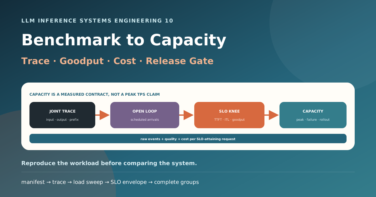
오늘의 결론

• tokens/s 하나에는 workload, batch, prompt·output 길이, SLO와 cache 상태가 없습니다. Benchmark 결과는 system manifest + workload trace + load model + metric contract와 함께만 의미가 있습니다.
• Production capacity는 open-loop arrival로 측정합니다. Server가 느려질수록 client도 요청을 덜 보내는 closed-loop만 사용하면 queue collapse와 coordinated omission을 숨길 수 있습니다.
• Input과 output 길이는 따로 random sampling하지 않습니다. 둘의 결합 분포, prefix·session locality, tenant·SLO class, Agent fan-out을 보존한 trace를 같은 tokenizer revision으로 재생합니다.
• Offered load를 올리며 TTFT·ITL attainment가 유지되는 마지막 지점, 즉 SLO capacity envelope를 찾습니다. Peak throughput이 아니라 goodput의 saturation knee가 replica당 capacity입니다.
• 필요한 GPU는 평균 RPS를 peak token/s로 나눠 구하지 않습니다. Peak trace, forecast error, complete-group failure, rollout, cold-start·autoscaling gap을 더하고 cost와 quality gate까지 통과시킵니다.

앞 글에서는 SLO admission·fairness·autoscaling control loop를 설계했습니다. 이번 글은 그 controller가 사용할 capacity 숫자를 어떻게 만들고, engine 변경을 어떤 증거로 release할지를 다룹니다.

freeze system identity and metric semantics
  → build a production-shaped trace
  → replay arrivals without self-throttling
  → sweep load through saturation
  → measure latency, goodput, memory, fairness, failure, cost
  → derive complete-group capacity and headroom
  → publish raw events, manifest, report, and release decision

이 글에서 답하는 질문

1. Offline·closed-loop·open-loop benchmark는 무엇을 측정하는가?
2. Input/output 결합 분포와 prefix locality를 왜 trace에 보존해야 하는가?
3. TTFT·ITL·TPOT·throughput·goodput을 어떤 timestamp와 denominator로 계산하는가?
4. Coordinated omission과 load-generator bottleneck을 어떻게 찾는가?
5. SLO capacity envelope에서 필요한 replica·GPU·failure headroom을 어떻게 계산하는가?
6. 비용·에너지·quality·failure를 포함한 release gate는 어떻게 만드는가?

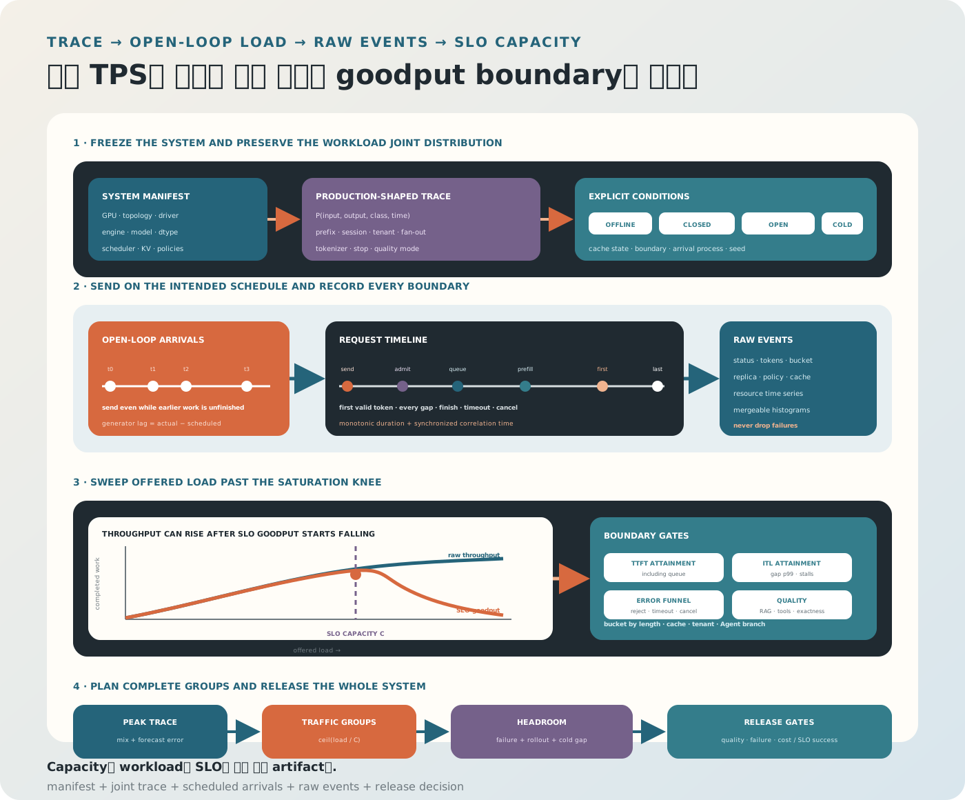
그림 1. Capacity는 하드웨어 속성이 아니라 특정 workload·SLO·software stack의 측정값이다. Manifest와 raw event가 없으면 같은 그래프를 다시 만들 수도, regression 원인을 설명할 수도 없다.

---

1. 먼저 Benchmark 질문을 한 문장으로 쓴다

다음 질문은 서로 다른 실험입니다.

• 한 request의 가장 빠른 decode rate는 얼마인가?
• SLO 없이 GPU가 생성할 수 있는 최대 output token/s는 얼마인가?
• TTFT 2초·ITL 80ms를 99% 만족하는 최대 offered RPS는 얼마인가?
• Production trace peak에 필요한 replica와 failure reserve는 몇 개인가?
• 두 GPU·engine 조합 중 SLO를 만족하는 request당 비용이 낮은 것은 무엇인가?

질문 없이 config부터 sweep하면 가장 보기 좋은 숫자를 고르게 됩니다. Decision, population, constraint와 objective를 실험 계획에 적습니다.

2. 측정 Boundary를 고정한다

Kernel Microbenchmark

GEMM·attention·collective 같은 primitive를 측정합니다. 원인 분석에는 좋지만 service capacity는 아닙니다.

Engine Benchmark

Tokenizer·HTTP를 제외한 prefill·decode runtime을 측정합니다. Scheduler·KV·batch 효과를 볼 수 있습니다.

Serving Benchmark

Gateway부터 streaming response까지 측정합니다. Routing·queue·serialization·network가 포함됩니다.

End-to-end RAG Agent

Retrieval, reranking, prompt assembly, LLM, tool, validation을 모두 포함합니다. 사용자 SLO와 가장 가깝지만 LLM 원인을 분리할 stage trace가 필요합니다.

결과 표에 boundary를 반드시 표시합니다. Engine TTFT와 client-observed TTFT를 같은 열에서 비교하지 않습니다.

3. System under Test를 얼린다

최소 manifest:

hardware:
  gpu: "<model, count, memory, power limit, clocks>"
  topology: "<PCIe, NVLink, NIC, NUMA>"
  cpu_memory_network: "<spec>"
software:
  os_kernel_driver_firmware: "<versions>"
  cuda_rocm: "<version>"
  engine_commit_image_digest: "<immutable IDs>"
model:
  id_revision_tokenizer: "<immutable IDs>"
  dtype_quant_recipe: "<manifest>"
runtime:
  tp_pp_ep_cp: [1, 1, 1, 1]
  scheduler: "<all knobs>"
  kv_cache: "<dtype, block, capacity>"
  graph_compile: "<mode and buckets>"
control_plane:
  admission_fairness_autoscaler: "<policy revisions>"

GPU 이름과 model 이름만으로는 재현되지 않습니다. Power limit, driver, engine commit, quantized pack format과 scheduler default가 결과를 바꿉니다.

4. 환경 Noise도 Workload다

다음 조건을 기록하거나 격리합니다.

• Shared GPU·MIG·host process
• CPU governor·NUMA·IRQ placement
• GPU clock·thermal throttling·ECC
• Network contention·packet loss·NIC affinity
• Remote storage·weight cache traffic
• Telemetry profiler overhead
• Region 간 client RTT
• Cloud noisy neighbor와 preemption

완전히 제거할 수 없으면 production-like interference 시나리오로 별도 측정합니다. 조용한 lab 숫자와 noisy production capacity를 섞지 않습니다.

5. Workload Trace Contract

Request 하나에 다음을 보존합니다.

{
  "trace_id": "tr_...",
  "scheduled_offset_ms": 1832,
  "tenant_class": "interactive_standard",
  "model_revision": "model-v3",
  "adapter_id": null,
  "input_tokens": 8420,
  "max_output_tokens": 512,
  "observed_output_tokens": 286,
  "slo_ms": {"ttft": 2000, "itl": 80},
  "prefix_group": "policy-manual-v7",
  "session_group": "session-...",
  "agent_root": "root-...",
  "branch_depth": 1,
  "stop_policy": "stop-v2"
}

원문 prompt를 저장할 수 없으면 token-length·prefix grouping·approved synthetic template로 privacy-preserving trace를 만듭니다. Length만 같아도 speculative acceptance, MoE routing, structured decoding은 달라질 수 있음을 limitation에 적습니다.

6. Tokenizer Revision을 고정한다

문자 수나 단어 수는 GPU work 단위가 아닙니다. 같은 text도 tokenizer와 chat template에 따라 token 수가 달라집니다.

• System·developer·tool schema를 포함한 최종 prompt를 tokenize합니다.
• BOS/EOS·special token을 포함하는지 명시합니다.
• Prompt cache에 들어간 prefix도 logical input token과 computed token을 나눕니다.
• Output token은 server usage와 client retokenization 중 source of truth를 정합니다.
• Reasoning token·hidden token이 별도 과금/compute라면 trace schema에 둡니다.

Model revision과 tokenizer revision을 분리해 보존합니다.

7. Input과 Output은 결합 분포다

P(input)과 P(output)을 각각 뽑아 무작위로 조합하면 production에 없던 요청을 만듭니다.

customer support: medium input → short grounded answer
summarization: long input → medium output
reasoning: short/medium input → very long output
tool call: long schema input → tiny JSON output

필요한 것은 P(input, output, class, prefix, time)의 근사입니다. Joint histogram이나 실제 anonymized row를 sampling합니다. Long-tail과 correlation을 유지합니다.

8. Output 길이를 어떻게 재현할까

Generation은 model·sampling·stop 조건에 따라 달라집니다.

Natural Generation

실제 prompt와 decoding policy로 생성합니다. Quality와 현실성은 높지만 run별 output 길이가 달라 비교 분산이 생깁니다.

Forced Length

EOS를 무시하거나 synthetic token을 사용해 지정 길이를 생성합니다. Kernel·scheduler capacity 비교에는 좋지만 실제 stop·quality behavior를 잃습니다.

Recorded Replay Bucket

Production output length 분포에 맞춘 prompt template와 output cap을 사용합니다.

성능 microbenchmark와 quality-preserving service benchmark를 분리하고 어떤 mode인지 명시합니다.

9. Prefix와 Session Locality

Prefix cache를 켠 채 prompt를 모두 무작위로 만들면 hit가 0%이고, 같은 prompt만 반복하면 거의 100%입니다. 둘 다 production과 다를 수 있습니다.

Trace에 보존할 것:

• Shared system/tool prefix ID와 길이
• Session turn 순서와 inter-arrival gap
• Tenant별 template distribution
• Router stickiness
• Cache capacity·TTL·eviction
• Cold reset·warm state

Report에는 logical input tokens, actually computed prefill tokens, cache hit token과 cache memory를 함께 둡니다.

10. 세 가지 Load Model

Offline

모든 sample이 준비된 상태에서 최대한 처리합니다. Peak throughput·batch efficiency를 측정하며 user latency SLO는 목적이 아닙니다.

Closed-loop

고정 concurrency client가 응답을 받은 뒤 다음 요청을 보냅니다.

send → wait response → optional think time → send next

Interactive session과 single-user latency를 재현하기 좋지만 server가 느려질수록 offered rate도 내려갑니다.

Open-loop

응답과 무관하게 미리 정한 arrival schedule대로 보냅니다.

t0 send A
t0 + Δ1 send B even if A is unfinished
t0 + Δ2 send C

Production arrival rate와 overload capacity를 측정할 때 기본입니다. MLPerf Inference도 Offline과 Server 같은 scenario를 구분하며 LLM server에서 TTFT·TPOT constraint를 사용합니다.

11. Arrival Process를 명시한다

같은 평균 RPS라도 burstiness가 다르면 queue tail이 달라집니다.

• Constant interval
• Poisson/exponential inter-arrival
• Markov-modulated burst
• Production timestamp replay
• Diurnal scaled trace
• Tenant-correlated fan-out

정상 traffic capacity에는 production timestamp segment가 가장 직접적입니다. What-if sweep은 같은 trace의 time axis를 압축·확장해 request mix를 유지합니다.

12. Coordinated Omission

Load generator가 응답을 기다리느라 다음 요청을 늦게 보내면, 느린 시간대에 도착했어야 할 요청이 사라집니다. Tail latency가 실제보다 좋아 보입니다.

각 요청에 저장합니다.

t_scheduled: trace가 의도한 arrival
t_send:      generator가 실제 전송한 시각
t_server:    gateway가 받은 시각
t_first:     client가 첫 유효 token을 받은 시각
t_end:       마지막 유효 token을 받은 시각

Generator lag t_send - t_scheduled가 커지면 client가 bottleneck입니다. Capacity latency는 의도한 arrival를 기준으로 한 값과 실제 send 기준 값을 둘 다 보고합니다. wrk2는 intended schedule을 반영해 coordinated omission을 다루는 대표 도구의 설계 사례입니다.

13. Load Generator도 System이다

Generator가 CPU·socket·JSON parse·tokenizer에서 포화되면 target load를 못 보냅니다.

검사:

• Scheduled vs actual send rate
• Generator CPU·event loop lag
• Open connection·file descriptor
• NIC throughput·packet loss
• Client-side tokenization time
• SSE parse와 response buffering
• Client read backpressure
• Multiple generator의 clock·trace partition

Generator를 여러 machine으로 나누면 request ID와 scheduled clock을 일관되게 유지하고 target service와 network path를 기록합니다.

14. Clock과 Timestamp 의미

한 process 안 duration에는 monotonic clock을 사용합니다. 여러 host timestamp를 비교하려면 clock synchronization 오차를 측정합니다.

권장 event:

1. Scheduled arrival
2. Client send
3. Gateway receive
4. Admission decision
5. Engine enqueue
6. Prefill start/end
7. First decode start
8. First non-empty token client receive
9. 각 output token 또는 chunk receive
10. Last token·finish reason
11. Cancel·timeout·error

Wall clock은 trace correlation에, monotonic duration은 latency 계산에 사용합니다.

15. TTFT 정의

Client-observed TTFT:

$$ TTFT_i=t^{first\ valid\ token}_i-t^{arrival}_i $$

arrival은 production에서는 client send 또는 gateway receive, open-loop capacity에서는 intended scheduled time까지 별도 계산할 수 있습니다.

HTTP header, 빈 SSE heartbeat, role-only delta를 first token으로 세지 않습니다. 첫 사용자-visible text·tool token의 정의를 parser version과 함께 고정합니다.

16. ITL과 TPOT 정의

Token-level timestamp가 있다면:

$$ ITL_{i,j}=t_{i,j}-t_{i,j-1} $$

첫 token 이후 평균 TPOT의 한 정의:

$$ TPOT_i=\frac{t^{last}_i-t^{first}_i}{O_i-1} $$

O_i < 2 처리 규칙을 정합니다. 한 SSE chunk에 여러 token이 담기면 client arrival만으로 token별 ITL을 복원할 수 없습니다. Engine token timestamp 또는 chunk latency임을 명시합니다.

평균 TPOT 외에 ITL p95·p99, maximum stall, SLO를 넘긴 gap 비율을 봅니다.

17. Throughput 지표를 분리한다

Measurement duration T에서:

$$ request\ throughput=\frac{N_{completed}}{T} $$

$$ output\ throughput=\frac{\sum_i O_i}{T} $$

$$ total\ token\ throughput=\frac{\sum_i(P_i+O_i)}{T} $$

여기서 P_i가 logical input인지 computed input인지 명시합니다. Output token/s/GPU와 single-user decode token/s를 같은 “TPS”로 부르지 않습니다.

18. Goodput Envelope

SLO attainment target을 만족하는 최대 offered load를 찾습니다.

$$ C_{SLO}=\max_{\lambda}\left{\lambda: A_{TTFT}(\lambda)\ge a_t, A_{ITL}(\lambda)\ge a_i, E(\lambda)\le e \right} $$

• a_t, a_i: TTFT·ITL attainment 목표
• e: error·reject 상한

Load가 증가하면 처음에는 batching 덕분에 throughput이 좋아질 수 있습니다. 어느 지점부터 queue와 batch interference로 tail이 증가하고, peak throughput은 더 올라가도 SLO goodput은 떨어집니다. 이 saturation knee를 capacity로 사용합니다.

19. Load Sweep 방법

1. 낮은 offered load에서 baseline을 잡습니다.
2. 같은 trace mix로 rate를 단계적으로 높입니다.
3. 각 point에서 warm-up 후 충분한 steady window를 측정합니다.
4. SLO boundary 근처는 더 촘촘하게 sweep합니다.
5. 독립 repeat와 다른 trace segment로 재실행합니다.
6. Overload point도 지나가 queue collapse·recovery를 봅니다.
7. Scale-out을 켠 실험은 별도 dynamic trace로 수행합니다.

Binary search만 쓰면 noisy attainment 때문에 boundary가 흔들릴 수 있습니다. Monotonicity 위반과 confidence interval을 확인합니다.

20. Warm-up, Steady State, Cool-down

Warm-up

Weight page, allocator, JIT kernel, CUDA Graph, NCCL, prefix cache가 준비됩니다.

Steady State

Arrival·queue·memory가 목표 workload의 안정된 분포를 이룹니다. 이 구간의 event를 primary metric에 사용합니다.

Cool-down

Measurement 종료 시 이미 admitted된 요청이 끝나도록 합니다. 새 arrival를 멈춘 뒤 completion을 처리하지 않으면 long request가 denominator에서 사라집니다.

Warm-up sample을 버렸다면 얼마나, 왜 버렸는지 명시합니다. Cold-start benchmark에서는 버리지 않습니다.

21. Cache Condition을 네 Scenario로 나눈다

Cold Model

Process·weight가 없는 상태부터 ready까지 측정합니다.

Warm Model, Cold KV/Prefix

Kernel은 준비됐지만 request cache는 비어 있습니다.

Production Warm Cache

Trace와 eviction policy가 만든 정상 hit distribution을 사용합니다.

Adversarial Cache

Tenant churn·unique prefix·cache pollution을 재생합니다.

결과에 단순 cache=on 대신 state, capacity, TTL, preconditioning trace를 적습니다.

22. Percentile을 평균내지 않는다

Replica별 p99를 평균하면 cluster p99가 아닙니다. Request raw event나 merge 가능한 histogram을 합쳐 전체 distribution에서 percentile을 계산합니다.

주의:

• p99는 sample이 적으면 불안정합니다.
• Time-correlated burst는 iid bootstrap 가정을 깨뜨릴 수 있습니다.
• Trace segment별 repeat와 block bootstrap을 고려합니다.
• Mean·median·p95·p99·max를 함께 보되 SLO와 연결합니다.
• Histogram range·significant digits·overflow를 기록합니다.

Dean과 Barroso의 The Tail at Scale이 강조하듯 fan-out service는 component tail을 사용자 경로에서 증폭시킵니다.

23. Bucket별 Regression을 본다

전체 평균이 좋아도 특정 population이 나빠질 수 있습니다.

• Input length bucket
• Output length bucket
• Joint input/output quadrant
• TTFT·ITL SLO class
• Prefix hit/miss
• Tenant·priority
• Model·adapter
• Dense/MoE routing shape
• Structured output·speculative acceptance
• RAG Agent branch depth

Bucket sample 수와 confidence를 같이 보여 줍니다. 너무 세분화해 희소해지면 상위 class로 합칩니다.

24. Error, Timeout, Cancel도 결과다

다음을 latency dataset에서 조용히 제거하지 않습니다.

• Admission reject
• Queue timeout
• OOM·KV allocation failure
• Engine·rank crash
• Malformed stream·missing finish reason
• Client timeout·disconnect
• Cancel propagation delay
• Retry·duplicate completion

Offered, admitted, started, first-token, completed population을 funnel로 표시합니다. 성공한 빠른 요청만으로 p99를 계산하면 overload를 숨깁니다.

25. Quality를 같은 Run에 묶는다

Quantization·speculative decoding·model routing·structured kernel은 성능과 output을 바꿀 수 있습니다.

Quality gate:

• Model task·perplexity·long-context
• RAG groundedness·citation ID
• Tool name·argument exact match
• JSON schema validity
• 숫자·단위·날짜
• Safety·ACL·abstention
• Lossless decoding token equality가 요구되는 최적화

성능 결과에는 통과한 model·quality artifact hash를 연결합니다. Quality가 다른 model의 TPS를 같은 system 성능 비교로 해석하지 않습니다.

26. Fairness와 Multi-tenant Test

Aggregate goodput이 좋아도 한 tenant가 굶을 수 있습니다.

Trace에 heavy·light tenant, burst, priority를 포함하고 측정합니다.

• Tenant별 admitted work·completed work
• Weighted service share deviation
• Queue age·starvation max
• High-priority latency와 victim regression
• Work-conserving idle-share borrowing
• KV byte-seconds와 prefix cache share

앞 글의 fairness cost를 그대로 event log에서 재계산해 scheduler 구현과 맞는지 검증합니다.

27. Autoscaling Benchmark는 Timeline이다

Static capacity test와 분리합니다.

normal load
  → burst begins
  → desired replica increases
  → GPU provisioned
  → weight loaded / rank formed / warmed
  → router ready
  → queue recovers
  → scale-in drain

측정:

• Detection delay·decision delay
• Provision·load·warm·register time
• Burst 중 reject·SLO goodput
• Overshoot GPU-hours
• Scale thrash·partial group
• Recovery time와 queue area
• Downscale drain·cache loss

Cold-start보다 짧은 spike에는 warm floor와 admission이 실제로 작동하는지 확인합니다.

28. Failure와 Rollout Benchmark

정상 steady state에서 다음 fault를 주입합니다.

• GPU rank process 종료
• NIC bandwidth 제한·packet loss
• One node removal
• Prefix cache flush
• Weight store slowdown
• Control-plane metric stale
• Canary revision의 kernel fallback
• Rolling update 중 old/new capacity overlap

관찰할 것:

• Detection·route removal time
• In-flight stream failure·duplicate
• Retry amplification
• Complete-group capacity loss
• TTFT·ITL goodput recovery
• State·KV cleanup

Failure reserve는 이 실험에서 SLO가 유지되는 최소 group 수로 정합니다.

29. Memory Capacity의 시작 Bound

GPU당 KV에 쓸 수 있는 memory:

$$ M_{KV,budget}=M_{GPU}-M_{weight}-M_{runtime}-M_{graph}-M_{comm}-M_{reserve} $$

요청당 예약 KV의 chosen quantile이 M_KV,p라면 단순 upper bound:

$$ N_{seq}\lesssim\left\lfloor\frac{M_{KV,budget}}{M_{KV,p}}\right\rfloor $$

실제로는 sequence 길이가 섞이고 paged allocation·prefix sharing·output reservation이 있으므로 trace replay에서 allocation failure와 fragmentation을 측정합니다. 평균 KV만 사용하면 long-tail request가 OOM을 만듭니다.

30. Replica당 SLO Capacity

특정 workload trace, hardware, engine, SLO에서 측정한 C_SLO가 replica당 capacity입니다.

C_SLO is not portable across:
  model / tokenizer / quantization
  prompt-output distribution
  prefix hit and scheduler
  TP/PP topology
  TTFT/ITL target

Vidur 같은 simulation framework는 넓은 config 탐색 비용을 줄일 수 있습니다. 하지만 simulation predictor를 target hardware microprofile과 실제 serving point로 calibration하고 경계 근처를 실측합니다.

31. Peak Traffic에서 Base Replica 계산

Peak window의 offered rate λ_peak, forecast uncertainty u, replica당 SLO capacity C_SLO라면 시작점:

$$ R_{traffic}=\left\lceil\frac{\lambda_{peak}(1+u)}{C_{SLO}}\right\rceil $$

RPS 대신 workload mix를 보존한 trace multiplier로 구하는 편이 더 정확합니다. Peak가 long prompt·reasoning mix 변화와 함께 오면 평균-day C_SLO를 그대로 쓰지 않습니다.

32. Headroom을 Additive GPU Percent로 두지 않는다

계획 capacity는 complete replica group 단위입니다.

R_plan
  = traffic groups
  + largest required failure-domain reserve
  + rollout overlap groups
  + cold-start / forecast gap reserve

조건으로 표현하면 더 명확합니다.

capacity after one allowed failure
  ≥ peak offered workload at target SLO

capacity during max rollout surge
  ≥ peak workload + canary isolation

30% headroom보다 “node 1개 또는 zone 1개를 잃어도 어떤 SLO를 지키는가”가 검증 가능합니다.

33. Prefill/Decode Pool Capacity

P/D 분리에서는 하나의 RPS capacity로 부족합니다.

prefill demand:
  input shape · prefix miss · chunk work · TTFT target

decode demand:
  output distribution · active KV · ITL target

transfer demand:
  KV bytes · topology · overlap · queue

Trace에서 phase work를 분해해 P:D pool ratio를 sweep합니다. 한쪽의 local goodput이 아니라 request가 두 phase를 완료한 end-to-end goodput을 최적화합니다.

34. Heterogeneous GPU Capacity

GPU A가 GPU B보다 token/s가 높아도 비용 효율이 항상 높은 것은 아닙니다.

각 hardware·phase·shape에서:

• SLO capacity/GPU
• Cost/GPU-hour
• Power·energy
• Model fit·parallel degree
• Ready time·availability
• Network·KV transfer

를 측정합니다. Splitwise는 prefill과 decode 특성에 맞춘 homogeneous·heterogeneous cluster 설계를 다루고, DynamoLLM은 SLO 아래 energy·cost reconfiguration 관점을 제시합니다.

35. Cost의 Denominator

총 service 비용:

GPU + CPU + host memory
+ network + storage + observability
+ idle warm capacity + failed / warming groups
+ data transfer + managed control plane

권장 지표:

$$ Cost_{req}=\frac{total\ cost}{SLO\ satisfying\ requests} $$

$$ Cost_{1Mtok}=\frac{total\ cost}{SLO\ satisfying\ output\ tokens}\times10^6 $$

Rejected·timed-out work가 사용한 비용도 numerator에 남습니다. 단순 output token 비용은 긴 input이 비싼 RAG workload를 숨길 수 있어 class별 request cost도 함께 봅니다.

36. Energy와 Carbon

측정 가능한 범위에서:

• GPU·node power sample interval
• Idle baseline
• Warm-up·model loading energy
• Joule per input/output token
• Joule per SLO-attaining request
• Peak power와 rack constraint

를 기록합니다. Software-reported board power와 facility energy는 boundary가 다릅니다. PUE·carbon intensity를 사용한다면 region·time source를 명시하고 performance artifact와 분리해 갱신합니다.

37. RAG Agent End-to-end Capacity

LLM engine이 100 RPS를 받아도 retrieval·tool이 40 RPS면 제품 capacity는 40 RPS 이하입니다.

Root request trace:

root arrival
  → retrieval fan-out / rerank
  → prompt build
  → LLM planning
  → tool wait
  → resume / repair / verifier branches
  → final grounded response

측정:

• Root TTFT·completion·success
• Stage latency·queue·fan-out
• LLM child calls/root와 token/root
• Cancel 후 낭비된 child work
• Citation·tool contract quality
• Root goodput/GPU-hour

Engine capacity와 application capacity를 함께 제공하되 서로 대체하지 않습니다.

38. Raw Request Event를 보존한다

Summary CSV만 남기면 새로운 SLO로 재계산할 수 없습니다.

{
  "request_id": "req_...",
  "trace_row": 1842,
  "scheduled_ns": 0,
  "sent_ns": 0,
  "server_received_ns": 0,
  "admitted_ns": 0,
  "prefill_start_ns": 0,
  "first_token_ns": 0,
  "last_token_ns": 0,
  "input_tokens": 8420,
  "computed_input_tokens": 1760,
  "output_tokens": 286,
  "finish_reason": "stop",
  "status": "completed",
  "tenant_class": "interactive_standard",
  "replica_group": "rg-17",
  "policy_revision": "slo-v3"
}

Token timestamp가 크면 compressed array·histogram을 별도 object로 두고 checksum을 연결합니다. Prompt·PII는 저장하지 않습니다.

39. Benchmark Artifact 묶음

run/
  manifest.yaml
  workload.schema.json
  workload.parquet
  raw-events.parquet
  token-gaps.hdr
  quality-report.json
  resource-timeseries.parquet
  failure-timeline.jsonl
  summary.json
  plots/
  reproduce.md
  checksums.txt

Code commit, container digest, command, random seed와 secret-free config를 포함합니다. Raw → summary → plot 변환 script도 version 관리합니다.

40. 비교 Report의 최소 표

항목	Baseline	Candidate	Delta	Gate
Offered RPS	동일	동일	0	exact
TTFT p99	측정	측정	%	≤ SLO
ITL p99	측정	측정	%	≤ SLO
Request goodput/GPU	측정	측정	%	no regression
Peak resident memory	측정	측정	%	no OOM
Reject·error	측정	측정	pp	≤ limit
Fair share deviation	측정	측정	pp	≤ limit
Quality contract	측정	측정	diff	pass
Cost/SLO request	측정	측정	%	improve
Failure recovery	측정	측정	%	≤ objective

같은 offered trace와 SLO가 아니라면 나란히 놓지 않고 별도 scenario로 표시합니다.

41. Release Gate를 층으로 나눈다

Correctness

• Model·tokenizer·API contract
• Streaming·finish·usage count
• Lossless optimization token equality

Quality

• General task와 RAG Agent field-level regression

Performance

• Target bucket TTFT·ITL·goodput
• Memory·kernel·collective fast path

Reliability

• Overload·failure·retry·rollout recovery

Economics

• Cost·energy per SLO success

앞 gate가 실패하면 뒤의 더 좋은 TPS로 덮지 않습니다. Exception은 owner·expiry·rollback 조건과 함께 승인합니다.

42. Continuous Performance Regression

모든 commit에 full cluster benchmark를 돌릴 필요는 없습니다.

per PR:
  unit + deterministic microbench + small shape smoke

nightly:
  engine trace subset + quality + key GPU shapes

release candidate:
  full open-loop sweep + failure + cost

periodic production calibration:
  latest anonymized trace + hardware drift

Threshold 근처 noisy metric은 한 번의 run으로 fail/pass하지 않고 repeat·confidence와 known variance를 사용합니다. 그래도 OOM·wrong token·fallback 같은 deterministic failure는 즉시 막습니다.

43. Simulation과 실측의 역할

Simulation은 수백 개 parallelism·scheduler·hardware 조합을 빠르게 좁힐 수 있습니다. Vidur는 model execution profiling을 바탕으로 LLM inference simulation과 benchmark를 다룹니다.

하지만 predictor가 학습하지 않은 영역에서는 오차가 큽니다.

• 새 GPU·kernel·quantization
• Prefix cache·speculative acceptance 변화
• Network contention·failure
• Agent fan-out·structured decoding

Simulation으로 후보를 줄이고 SLO boundary, saturation knee, failure point는 실제 cluster에서 검증합니다. Predicted vs actual error를 다음 simulation calibration에 반영합니다.

44. Capacity Planning 예시 절차

1. 최근 production trace에서 peak와 normal segment를 선택합니다.
2. PII를 제거하고 joint input/output·prefix·tenant·SLO를 보존합니다.
3. Candidate system manifest와 quality artifact를 고정합니다.
4. Single-request·offline으로 correctness와 upper bound를 확인합니다.
5. Open-loop로 normal trace rate를 sweep합니다.
6. TTFT·ITL·error gate가 유지되는 C_SLO를 찾습니다.
7. Peak mix가 다르면 peak trace로 다시 envelope를 만듭니다.
8. Cache cold/warm·P/D ratio·failure domain을 별도 sweep합니다.
9. Forecast error를 포함해 traffic group 수를 계산합니다.
10. Node/zone failure와 rollout 중 capacity 조건을 만족하는 reserve를 더합니다.
11. Dynamic burst에서 autoscaling ready time과 queue recovery를 검증합니다.
12. Root RAG Agent quality·goodput과 cost로 최종 release합니다.

45. 이 시리즈의 연결 지도

단계	글	Capacity artifact에 남는 것
1	GPU Roofline	Compute·bandwidth 병목 가설
2	Memory Accounting	Weight·KV·workspace ledger
3	Transformer Kernel	Kernel timeline·fusion
4	Continuous Batching	Scheduler·chunk config
5	Paged KV·Prefix Cache	KV capacity·locality·eviction
6	Speculative Decoding	Acceptance·target step·quality
7	Distributed Inference	Rank map·collective·KV transfer
8	Low Precision	Dtype·scale·packed kernel artifact
9	SLO Operations	Admission·fairness·autoscaling policy
10	현재 글	Trace·goodput envelope·capacity decision

각 최적화는 독립된 “속도 팁”이 아니라 같은 run manifest와 release gate 안에서 상호작용합니다.

실전 체크리스트

• Benchmark가 답할 decision과 boundary를 먼저 적었다.
• Hardware·topology·driver·engine·model revision을 고정했다.
• Scheduler·KV·quantization·parallel config를 모두 보존했다.
• Input/output·tenant·SLO·prefix의 결합 분포를 유지했다.
• Tokenizer·chat template·stop policy가 동일하다.
• Natural generation과 forced-length test를 구분했다.
• Offline·closed-loop·open-loop 결과를 섞지 않는다.
• Arrival process와 random seed·trace segment를 기록했다.
• Scheduled·actual send time으로 coordinated omission을 확인했다.
• Load generator CPU·network·event-loop lag가 충분한 headroom을 가진다.
• TTFT 첫 유효 token과 ITL/TPOT 정의가 명시돼 있다.
• Request·input·output·computed token throughput을 구분했다.
• Offered·admitted·completed·error denominator를 모두 본다.
• Load sweep이 saturation knee와 overload recovery를 포함한다.
• Warm-up·steady·cool-down population을 구분했다.
• Model cold·KV cold·production warm cache를 따로 측정했다.
• Raw event를 합쳐 percentile을 계산하고 p99를 평균내지 않는다.
• Length·cache·tenant·Agent bucket별 regression을 확인했다.
• Quality와 performance artifact가 같은 model revision을 가리킨다.
• Autoscaling ready timeline과 failure·rollout을 benchmark했다.
• Complete-group failure reserve 뒤에도 peak SLO를 만족한다.
• Cost·energy denominator가 SLO-attaining request/token이다.
• Raw event·manifest·reproduce command·checksum을 보존했다.

스스로 확인하기

Q1. Offline output token/s가 가장 높은 설정을 production에 쓰면 되는가?

아닙니다. Offline은 모든 work가 준비된 최대 throughput scenario입니다. Online production에서는 arrival, queue, TTFT·ITL, KV residency와 fairness가 있습니다. Open-loop SLO goodput envelope를 별도로 측정해야 합니다.

Q2. Concurrency 100 closed-loop test가 100명의 user를 재현하는가?

일부 interactive workload에는 도움이 되지만 server가 느려지면 각 client의 다음 요청도 늦어져 offered load가 감소합니다. 독립적으로 도착하는 production burst capacity는 scheduled open-loop trace로 측정합니다.

Q3. 평균 prompt 2K, 평균 output 200이면 그 두 길이로 benchmark해도 되는가?

아닙니다. 평균은 long-tail과 input/output correlation을 지웁니다. 32K prompt와 4K reasoning이 memory·tail을 지배할 수 있으므로 joint distribution과 quantile bucket을 보존합니다.

Q4. Replica당 20 RPS이고 peak가 100 RPS면 5 replicas면 충분한가?

그 20 RPS가 같은 peak workload·SLO에서 측정한 C_SLO인지 먼저 확인해야 합니다. Forecast error, complete-group failure, rollout overlap과 cold-start gap을 더하고, failure 후에도 peak SLO를 지키는지 trace replay로 검증합니다.

Q5. Candidate가 20% 빠르지만 RAG citation exact match가 떨어지면 release할 수 있는가?

기본적으로 안 됩니다. Quality와 correctness는 performance보다 앞선 gate입니다. 승인된 quality trade-off가 제품 계약에 명시된 경우만 owner·expiry·rollback 조건과 함께 예외로 다룹니다.

시리즈를 마치며

LLM inference는 GPU kernel 하나가 아니라 memory, scheduler, KV, decoding, parallelism, numerical format과 control plane이 이어진 시스템입니다. 이 10편의 최종 산출물은 “몇 token/s”가 아니라 다음의 재현 가능한 묶음입니다.

workload trace
+ model and system manifest
+ memory and execution timeline
+ SLO goodput capacity envelope
+ quality / failure / cost release gates

다음 학습은 LLM 추론 시스템 엔지니어링 시리즈 페이지에서 필요한 병목 축을 골라 반복하면 됩니다. 새 hardware·engine·model이 나와도 이 측정 계약을 유지하면 무엇이 실제로 개선됐는지 다시 증명할 수 있습니다. 이어서 Enterprise RAG 지식 수명주기에서는 Agent가 읽는 원문·chunk·index도 같은 manifest와 release gate로 운영합니다.

참고문헌

• Reddi et al., MLPerf Inference Benchmark, ISCA 2020.
• MLCommons, MLPerf Inference Benchmark Suite and Rules, accessed 2026-07-16.
• Agrawal et al., Vidur: A Large-Scale Simulation Framework for LLM Inference, MLSys 2024.
• Zhong et al., DistServe: Disaggregating Prefill and Decoding for Goodput-optimized Large Language Model Serving, OSDI 2024.
• Agrawal et al., Taming Throughput-Latency Tradeoff in LLM Inference with Sarathi-Serve, OSDI 2024.
• Sheng et al., Fairness in Serving Large Language Models, OSDI 2024.
• Gujarati et al., Serving DNNs like Clockwork: Performance Predictability from the Bottom Up, OSDI 2020.
• Dean and Barroso, The Tail at Scale, Communications of the ACM, 2013.
• Tene, wrk2: A Constant Throughput, Correct Latency Recording Variant of wrk, accessed 2026-07-16.
• Patel et al., Splitwise: Efficient Generative LLM Inference Using Phase Splitting, ISCA 2024.
• Stojkovic et al., DynamoLLM: Designing LLM Inference Clusters for Performance and Energy Efficiency, HPCA 2025.

검증 메모 — 개념과 문헌은 2026년 7월 16일 확인했습니다. Benchmark capacity는 workload·SLO·hardware·engine·policy revision에 종속되며 다른 환경으로 그대로 이전할 수 없습니다. 본문의 trace schema·식·gate는 시작 템플릿입니다. Production privacy policy에 맞춘 raw event와 독립 workload segment로 반복하고, capacity boundary·failure reserve·비용을 target cluster에서 다시 측정해야 합니다.